Chi-Square test of independence (R)
इस पोस्ट में, मैं Chi Square test of independence के बारे में बात करना चाहता हूँ। जो डेटा सेट मैं उपयोग करने जा रहा हूँ, वो https://smartcities.data.gov.in पर प्रकाशित है, जो कि भारत सरकार का एक प्रोजेक्ट है, जो National Data Sharing and Accessibility Policy के तहत आता है।
मैं जानना चाहता हूँ कि बैंगलोर की सड़कों पर यात्रा करने के लिए सबसे सुरक्षित और सबसे खतरनाक तरीके कौन से हैं। Injuries_and_Fatalities_Bengaluru_from_2016to2018.csv डेटा सेट में 2016 से 2018 के बीच बैंगलोर में कुल चोटों और मौतों की संख्या है। मैं चोटों को उन घटनाओं की संख्या के लिए एक डमी के रूप में लेना चाहता हूँ जो हुईं।
चूंकि मैं यह परीक्षण करना चाहता हूँ कि विभिन्न प्रकार के परिवहन के साथ मौतों में महत्वपूर्ण अंतर है या नहीं, शून्य और वैकल्पिक परिकल्पना इस प्रकार होगी:
\(H_0\): परिवहन का प्रकार मौतों से स्वतंत्र है
\(H_1\): परिवहन का प्रकार मौतों पर निर्भर है
नमूना डेटा सेट:
##                                                                   instance
## 1 2017 - Total Injuries - Other modes of road transport (auto, bus, lorry)
## 2                                       2018 - Total Fatalities - Bicycles
## 3                                   2017 - Total Fatalities - Two-wheelers
## 4                                     2018 - Total Fatalities - Pedestrian
## 5                                       2017 - Total Fatalities - Bicycles
##   count year             type                                        transport
## 1  1380 2017   Total Injuries Other modes of road transport (auto, bus, lorry)
## 2     9 2018 Total Fatalities                                         Bicycles
## 3    98 2017 Total Fatalities                                     Two-wheelers
## 4   276 2018 Total Fatalities                                       Pedestrian
## 5     8 2017 Total Fatalities                                         Bicycles
2017 के लिए contingency table इस प्रकार है:
contingency_table <- data %>% filter(year == 2017) %>%
  dplyr::select(type, transport, count) %>%
  spread(type, count)
library(kableExtra)
kable(contingency_table,
      caption = 'Contingency Table') %>%
  kable_styling(full_width = F) %>%
  column_spec(1, bold = T) %>%
  collapse_rows(columns = 1:2, valign = "middle") %>%
  scroll_box()
| transport | Total Fatalities | Total Injuries |
|---|---|---|
| Bicycles | 8 | 31 |
| Other modes of road transport (auto, bus, lorry) | 252 | 1380 |
| Pedestrian | 284 | 1346 |
| Two-wheelers | 98 | 1499 |
इसके लिए एक Mosaic plot इस प्रकार है:
library(ggmosaic)
ggplot(data = data) +
  geom_mosaic(aes(weight = count, x = product(transport), fill = type), na.rm=TRUE) +
  labs(x = 'Type of transport', y='%',  title = 'What type of transport to use') +
    theme_minimal()+theme(legend.position="bottom")
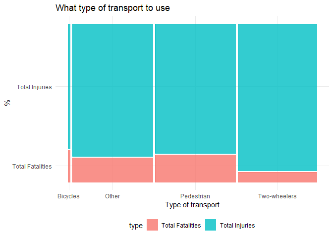
उपरोक्त प्लॉट से मैं देख सकता हूँ कि प्रत्येक परिवहन में मौतों के प्रतिशत में महत्वपूर्ण अंतर है। यह जानने के लिए कि यह प्रतिशत महत्वपूर्ण है या नहीं, मैं chi-square test of independence करूँगा।
library(gmodels)
# Converting contingency table to flat tables
# Two vectors to hold values of columns
caseType <- c();  conditionType <- c()

# For each cell, repeat the rowname, colname combo
# as many times
for(i in 1:nrow(contingency_table)) {
  for(j in 2:ncol(contingency_table)) {
    numRepeats <- contingency_table[i, j]

    caseType <- append(caseType,
                       rep(contingency_table[i,1],
                           numRepeats))
    conditionType <- append(conditionType,
                        rep(colnames(contingency_table)[j],
                            numRepeats))
  }
}

# Construct the table from the vectors
flatTable <- data.frame(caseType, conditionType)
CrossTable(flatTable$caseType, flatTable$conditionType,
           dnn=c("Transportation Type", "Accident type"),
           expected=TRUE)
##
##
##    Cell Contents
## |-------------------------|
## |                       N |
## |              Expected N |
## | Chi-square contribution |
## |           N / Row Total |
## |           N / Col Total |
## |         N / Table Total |
## |-------------------------|
##
##
## Total Observations in Table:  4898
##
##
##                                                  | Accident type
##                              Transportation Type | Total Fatalities |   Total Injuries |        Row Total |
## -------------------------------------------------|------------------|------------------|------------------|
##                                         Bicycles |                8 |               31 |               39 |
##                                                  |            5.112 |           33.888 |                  |
##                                                  |            1.632 |            0.246 |                  |
##                                                  |            0.205 |            0.795 |            0.008 |
##                                                  |            0.012 |            0.007 |                  |
##                                                  |            0.002 |            0.006 |                  |
## -------------------------------------------------|------------------|------------------|------------------|
## Other modes of road transport (auto, bus, lorry) |              252 |             1380 |             1632 |
##                                                  |          213.913 |         1418.087 |                  |
##                                                  |            6.782 |            1.023 |                  |
##                                                  |            0.154 |            0.846 |            0.333 |
##                                                  |            0.393 |            0.324 |                  |
##                                                  |            0.051 |            0.282 |                  |
## -------------------------------------------------|------------------|------------------|------------------|
##                                       Pedestrian |              284 |             1346 |             1630 |
##                                                  |          213.650 |         1416.350 |                  |
##                                                  |           23.164 |            3.494 |                  |
##                                                  |            0.174 |            0.826 |            0.333 |
##                                                  |            0.442 |            0.316 |                  |
##                                                  |            0.058 |            0.275 |                  |
## -------------------------------------------------|------------------|------------------|------------------|
##                                     Two-wheelers |               98 |             1499 |             1597 |
##                                                  |          209.325 |         1387.675 |                  |
##                                                  |           59.206 |            8.931 |                  |
##                                                  |            0.061 |            0.939 |            0.326 |
##                                                  |            0.153 |            0.352 |                  |
##                                                  |            0.020 |            0.306 |                  |
## -------------------------------------------------|------------------|------------------|------------------|
##                                     Column Total |              642 |             4256 |             4898 |
##                                                  |            0.131 |            0.869 |                  |
## -------------------------------------------------|------------------|------------------|------------------|
##
##
## Statistics for All Table Factors
##
##
## Pearson's Chi-squared test
## ------------------------------------------------------------
## Chi^2 =  104.4776     d.f. =  3     p =  1.692478e-22
##
##
##
chi.test <- chisq.test(contingency_table[,2:3], rescale.p = TRUE)
print(chi.test)
##
##  Pearson's Chi-squared test
##
## data:  contingency_table[, 2:3]
## X-squared = 104.48, df = 3, p-value < 2.2e-16
chi.sq.plot(chi.sq = chi.test$statistic, df = chi.test$parameter, title = 'Null hypothesis to test independence')
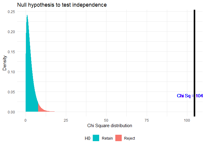
चूंकि \(p < \alpha\), जहाँ \(\alpha = 0.05\), मैं Null hypothesis को अस्वीकार करता हूँ। विभिन्न वाहनों के साथ मृत्यु दर में महत्वपूर्ण अंतर है। दो-पहिया वाहन पर यात्रा करना सबसे सुरक्षित है जबकि साइकिल सबसे खतरनाक है।