ARIMA in R

Arima model¶

ARIMA, जिसका पूरा नाम 'Auto Regressive Integrated Moving Average' है, एक बहुत ही लोकप्रिय forecasting model है। ARIMA models मूल रूप से regression models होते हैं: auto-regression का मतलब है एक variable का अपने आप पर regression, जो विभिन्न समय अवधियों में मापा जाता है।

AR: Autoregression. एक model जो एक observation और कुछ lagged observations के बीच निर्भरता का उपयोग करता है।
I: Integrated. कच्चे observations के differencing का उपयोग (यानी, एक observation को पिछले समय चरण के observation से घटाना) ताकि time series stationary हो सके।
MA: Moving Average. एक model जो एक observation और lagged observations पर लागू किए गए moving average model से residual errors के बीच निर्भरता का उपयोग करता है।

Stationary¶

AR model का अनुमान है कि time series एक stationary process है। यदि एक time-series data, $Y_t$, stationary है, तो यह निम्नलिखित शर्तों को पूरा करता है:
1. $Y_t$ के विभिन्न t मानों पर mean values स्थिर हैं।
2. विभिन्न समय अवधियों पर $Y_t$ के variances स्थिर हैं (Homoscedasticity)।
3. विभिन्न lags के लिए $Y_t$ और $Y_{t-k}$ के covariances केवल k पर निर्भर करते हैं और समय t पर नहीं।

Box-Jenkins method¶

प्रारंभिक ARMA और ARIMA models को Box और Jenkins ने 1970 में विकसित किया था। लेखकों ने किसी विशेष time series data-set के लिए models की पहचान, अनुमान और जांचने की प्रक्रिया भी सुझाई। इसमें तीन चरण शामिल हैं:

Model form selection
1.1 Stationarity का मूल्यांकन करें।
1.2 Differencing level (d) का चयन करें – stationarity समस्याओं को ठीक करने के लिए।
1.3 AR level (p) का चयन करें।
1.4 MA level (q) का चयन करें।
Parameter estimation
Model checking

Model form selection¶

Evaluate stationarity¶

एक stationary time series वह है जिसकी विशेषताएँ उस समय पर निर्भर नहीं करती हैं जब series का अवलोकन किया जाता है। Trends या seasonality वाले time series stationary नहीं होते हैं। एक white noise series stationary होती है — यह मायने नहीं रखता कि आप इसे कब अवलोकित करते हैं, यह किसी भी समय पर लगभग समान दिखनी चाहिए।

Stationarity की उपस्थिति कई तरीकों से पाई जा सकती है, जिनमें से सबसे लोकप्रिय तीन हैं:
1. ACF plot: जब data non-stationary होता है, auto-correlation function जल्दी से zero पर नहीं कटता।
2. Dickey−Fuller या augmented Dickey−Fuller tests।
3. KPSS test.

नीचे दिए गए उदाहरण में, मैं अपने attendance data set से एक sample का उपयोग करूंगा, जिसे EDA blogs में वर्णित किया गया है। (वास्तविक data को गोपनीयता कारणों से नहीं दिखाया गया है। यह mock data है जो वास्तविक data के बहुत समान है। विश्लेषण वही होगा।)

इसका time plot नीचे दिखाया गया है: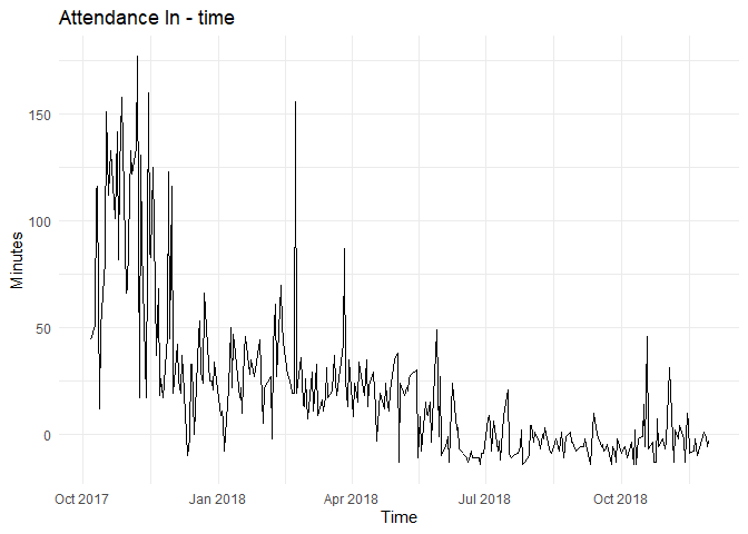

Plot को देखकर, मैं स्पष्ट रूप से देख सकता हूँ कि series stationary नहीं है क्योंकि trend स्पष्ट है और variance समय के साथ घटता हुआ प्रतीत होता है।
इस time series का ACF है:

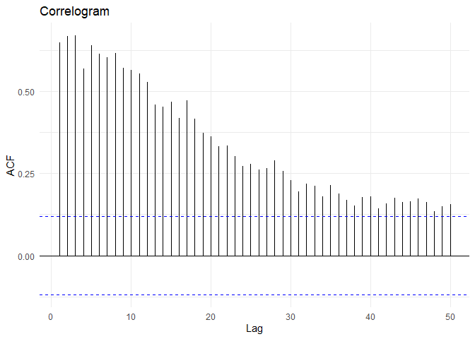
ऊपर दिए गए plot से, मैं पहचान सकता हूँ कि time series stationary नहीं है।

Augmented Dickey−Fuller Test¶

Augmented Dickey−Fuller test एक hypothesis test है जिसमें null hypothesis और alternative hypothesis इस प्रकार हैं:
$H_0$: $\gamma$ = 0 (time series non-stationary है)
$H_1$: $\gamma$ < 0 (time series stationary है)
जहाँ $\Delta y_t = \alpha + \beta t + \gamma y_{t-1} + \delta_1 \Delta y_{t-1} + \delta_2 \Delta y_{t-2} + \dots$

## 
##  Augmented Dickey-Fuller Test
## 
## data:  time.series
## Dickey-Fuller = -2.8819, Lag order = 6, p-value = 0.2045
## alternative hypothesis: stationary

चूंकि p value cutoff $ \alpha = 5\% $ से अधिक है, null hypothesis को बनाए रखा जा रहा है कि time series non-stationary है।

KPSS Test¶

KPSS test के लिए null hypothesis यह है कि data stationary है। इस test के लिए, हम null hypothesis को अस्वीकार नहीं करना चाहते हैं।

## 
##  KPSS Test for Trend Stationarity
## 
## data:  time.series
## KPSS Trend = 0.41839, Truncation lag parameter = 5, p-value = 0.01

चूंकि p-value 5% से कम है, हम null hypothesis को अस्वीकार कर रहे हैं कि data stationary है।

Selection of differencing parameter d¶

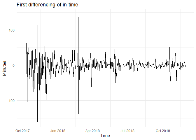
Attendance data (in time) ने stationary के लिए दोनों tests, Augmented Dickey-Fuller और KPSS test में असफलता प्राप्त की है। Differencing का उपयोग data को stationary model में परिवर्तित करने के लिए किया जाता है। Differencing का मतलब है लगातार observations के बीच के differences की गणना करना।

पहले difference के लिए in-time के लिए ऊपर दिए गए tests इस प्रकार दिखते हैं:

## 
##  Augmented Dickey-Fuller Test
## 
## data:  time.series.diff
## Dickey-Fuller = -10.851, Lag order = 6, p-value = 0.01
## alternative hypothesis: stationary

## 
##  KPSS Test for Trend Stationarity
## 
## data:  time.series %>% diff()
## KPSS Trend = 0.01895, Truncation lag parameter = 5, p-value = 0.1

d = 1 के द्वारा differencing के बाद, differenced in-time का ACF एक white noise series की तरह दिखता है। ADF test में p-value cutoff से कम है, null hypothesis को अस्वीकार करते हुए कि time series non-stationary है जबकि KPSS test का p-value 5% से अधिक है, null hypothesis को बनाए रखते हुए कि data stationary है। यह सुझाव देता है कि एक बार differencing के बाद, in-time मूलतः एक यादृच्छिक मात्रा है और stationary है।

## [1] "The ideal differencing parameter is 1"

## 
## ####################### 
## # KPSS Unit Root Test # 
## ####################### 
## 
## Test is of type: mu with 5 lags. 
## 
## Value of test-statistic is: 0.0188 
## 
## Critical value for a significance level of: 
##                 10pct  5pct 2.5pct  1pct
## critical values 0.347 0.463  0.574 0.739

Selection of AR(p) and MA(q) parameters¶

Forecasting में autoregressive model का उपयोग करने में एक महत्वपूर्ण कार्य model identification है, यानी p और q (lags की संख्या) का मान पहचानना।
AR(p) और MA(q) lags का चयन दो तरीकों से किया जा सकता है:
1. ACF और PACF functions
2. AIC या BIC coefficients

ACF और PACF coefficients¶

Auto-correlation वह correlation है जो $Y_t$ के विभिन्न समय अवधियों में मापा जाता है (उदाहरण के लिए, $Y_t$ और $Y_{t-1}$ या $Y_t$ और $Y_{t-k}$)। विभिन्न k मानों के लिए auto-correlation का एक plot auto-correlation function (ACF) या correlogram कहलाता है।
Lag k का partial auto-correlation वह correlation है जो $Y_t$ और $Y_{t-k}$ के बीच है जब सभी intermediate values ($Y_{t-1}$, $Y_{t-2}$...$Y_{t-k+1}$) का प्रभाव हटा दिया जाता है (partial out) दोनों $Y_t$ और $Y_{t-k}$ से। विभिन्न k मानों के लिए partial auto-correlation का एक plot partial auto-correlation function (PACF) कहलाता है।

Hypothesis tests किए जा सकते हैं यह जांचने के लिए कि क्या auto-correlation और partial auto-correlation के मान zero से भिन्न हैं। संबंधित null और alternative hypotheses हैं:
$H_0: r_k = 0$ और
$H_A: r_k \neq 0$,
जहाँ $r_k$ k के order का auto-correlation है।

$H_0: r_{pk} = 0$ और
$H_A: r_{pk} \neq 0$,
जहाँ $r_{pk}$ k के order का partial auto-correlation है।

Null hypothesis को तब अस्वीकार किया जाता है जब $|r_k| > \frac{1.96}{\sqrt{n}}$ और $|r_{pk}| > \frac{1.96}{\sqrt{n}}$। ACF और PACF plots में, यह cutoff dotted blue lines के रूप में दिखाया गया है।

ARMA process में p और q के मानों की पहचान निम्नलिखित thumb rule का उपयोग करके की जा सकती है:
1. Auto-correlation value, $r_p > cutoff$ पहले q मानों (पहले q lags) के लिए और zero पर कटता है।
2. Partial auto-correlation function, $r_{pk} > cutoff$ पहले p मानों के लिए और zero पर कटता है।

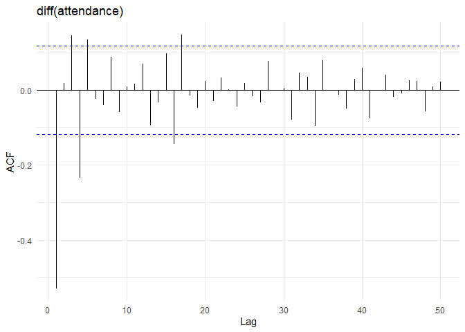
Differencing के बाद, in-time के ACF और PACF plots इस प्रकार हैं: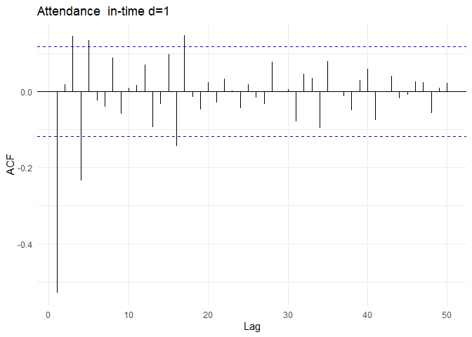

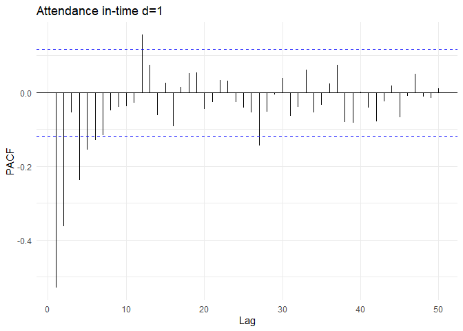
ACF और PACF plots से, auto-correlations पहले lag के बाद zero पर कट जाते हैं। PACF value 2 lags के बाद zero पर कट जाती है। इसलिए, उपयुक्त model ARMA(2, 1) process हो सकता है। पिछले अनुभाग से differencing parameter (d=1) को जोड़ते हुए, सबसे उपयुक्त model ARIMA(2, 1, 1) होगा।

AIC और BIC coefficients¶

Akaike’s Information Criterion (AIC) और Bayesian Information Criterion (BIC), जो regression के लिए predictors का चयन करने में उपयोगी होते हैं, ARIMA model के order को निर्धारित करने में भी उपयोगी होते हैं। AR और MA orders के सर्वोत्तम अनुमान AIC या BIC को कम करेंगे।

## 
##  Fitting models using approximations to speed things up...
## 
##  ARIMA(2,1,1) with drift         : 2503.652
##  ARIMA(0,1,0) with drift         : 2656.365
##  ARIMA(1,1,0) with drift         : 2569.569
##  ARIMA(0,1,1) with drift         : 2511.579
##  ARIMA(0,1,0)                    : 2654.343
##  ARIMA(1,1,1) with drift         : 2510.969
##  ARIMA(2,1,0) with drift         : 2526.337
##  ARIMA(3,1,1) with drift         : 2506.575
##  ARIMA(3,1,0) with drift         : 2523.835
##  ARIMA(2,1,1)                    : 2504.125
## 
##  Now re-fitting the best model(s) without approximations...
## 
##  ARIMA(2,1,1) with drift         : 2516.48
## 
##  Best model: ARIMA(2,1,1) with drift

## Series: time.series 
## ARIMA(2,1,1) with drift 
## 
## Coefficients:
##           ar1     ar2      ma1    drift
##       -0.0530  0.0200  -0.8174  -0.3120
## s.e.   0.0811  0.0751   0.0539   0.2595
## 
## sigma^2 estimated as 574.2:  log likelihood=-1253.13
## AIC=2516.26   AICc=2516.48   BIC=2534.3

AIC coefficient का उपयोग करके चयनित model ARIMA(2,1,1) है, जो ACF और PACF का उपयोग करके चयनित model के समान है।

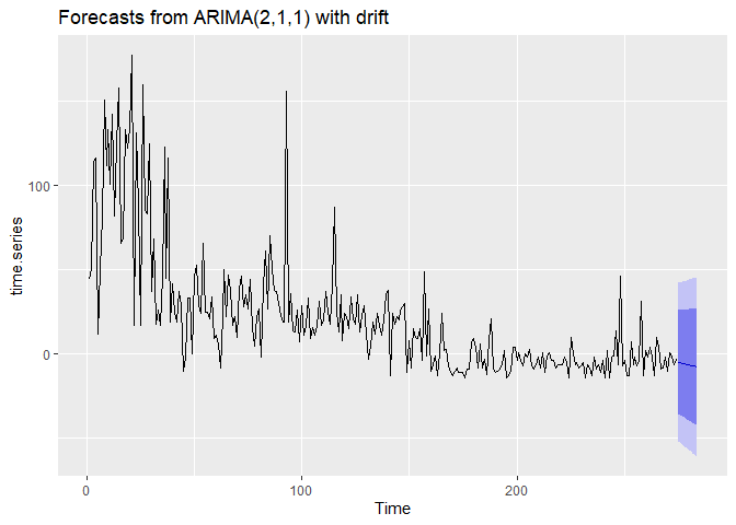
ARIMA(2, 1, 1) अंतिम model है जैसा कि दोनों तरीकों से चयनित किया गया है।

Parameter estimation¶

एक बार जब model order की पहचान हो जाती है (यानी, p, d और q के मान), तो हमें model parameters का अनुमान लगाने की आवश्यकता होती है। Parameters की पहचान के लिए regression model का उपयोग करते हुए:

## Series: time.series 
## ARIMA(2,1,1) with drift 
## 
## Coefficients:
##           ar1     ar2      ma1    drift
##       -0.0530  0.0200  -0.8174  -0.3120
## s.e.   0.0811  0.0751   0.0539   0.2595
## 
## sigma^2 estimated as 574.2:  log likelihood=-1253.13
## AIC=2516.26   AICc=2516.48   BIC=2534.3

Model testing¶

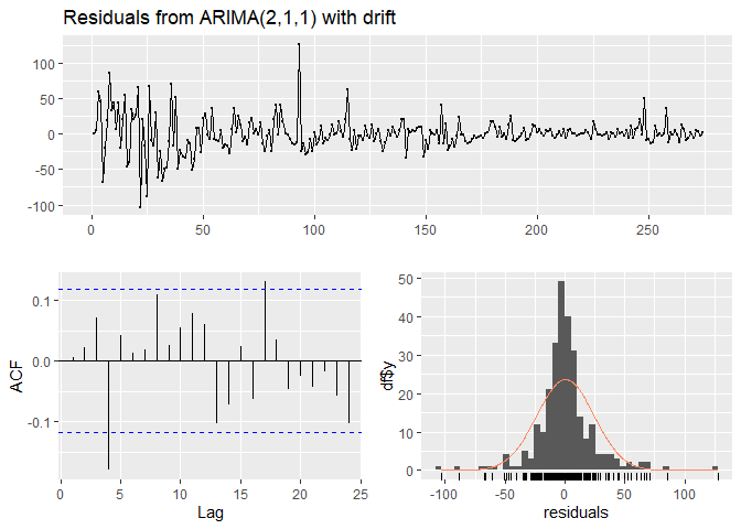
Residuals¶

Time series model में “residuals” वे होते हैं जो model को फिट करने के बाद बचे रहते हैं। Residuals यह जांचने में उपयोगी होते हैं कि क्या model ने data में जानकारी को उचित रूप से कैप्चर किया है। एक अच्छा forecasting method residuals के निम्नलिखित गुणों को उत्पन्न करेगा:
1. Residuals uncorrelated होते हैं। यदि residuals के बीच correlations हैं, तो residuals में कुछ जानकारी बची हुई है जिसे forecasts की गणना में उपयोग किया जाना चाहिए।
2. Residuals का mean zero होता है। यदि residuals का mean zero से अलग है, तो forecasts biased होते हैं।

Portmanteau tests for auto-correlation¶

जब हम ACF plot को देखते हैं यह देखने के लिए कि क्या प्रत्येक spike आवश्यक सीमाओं के भीतर है, तो हम निहित रूप से कई hypothesis tests कर रहे हैं, प्रत्येक एक छोटे false positive की संभावना के साथ। जब इन tests की संख्या पर्याप्त होती है, तो यह संभावना है कि कम से कम एक false positive देगा, और इसलिए हम निष्कर्ष निकाल सकते हैं कि residuals में कुछ शेष auto-correlation है, जबकि वास्तव में ऐसा नहीं है।

इस समस्या को दूर करने के लिए, हम यह परीक्षण करते हैं कि क्या पहले h auto-correlations white noise process से भिन्न हैं। Auto-correlations के एक समूह के लिए एक test को portmanteau test कहा जाता है। एक ऐसा test Ljung-Box test है।

Ljung−Box Test for Auto-Correlations¶

Ljung−Box एक forecasting model की lack of fit का test है और यह जांचता है कि क्या errors के लिए auto-correlations zero से भिन्न हैं। Null और alternative hypotheses इस प्रकार हैं:
$H_0$: Model lack of fit नहीं दिखाता।
$H_1$: Model lack of fit दिखाता है।
Ljung−Box statistic (Q-Statistic) इस प्रकार दिया गया है:
$$ Q(m) = n(n+2) \sum_{k=1}^{{m}\frac{\rho_k}2}{n-k} $$
जहाँ n time series में observations की संख्या है, k lag की संख्या है, $r_k$ lag k का auto-correlation है, और m कुल lags की संख्या है। Q-statistic एक अनुमानित chi-square distribution है जिसमें m – p – q degrees of freedom हैं जहाँ p और q AR और MA lags हैं।

## 
##  Ljung-Box test
## 
## data:  Residuals from ARIMA(2,1,1) with drift
## Q* = 15.754, df = 6, p-value = 0.01513
## 
## Model df: 4.   Total lags used: 10

ऊपर दिए गए tests से हम निष्कर्ष निकाल सकते हैं कि model data का अच्छा fit है।

References¶

Business Analytics: The Science of Data-Driven Decision Making - Dinesh Kumar
Forecasting: Principles and Practice - Rob J Hyndman और George Athanasopoulos - Online
SAS for Forecasting Time Series, Third Edition - Dickey
Applied Time Series Analysis for Fisheries and Environmental Sciences - E. E. Holmes, M. D. Scheuerell, और E. J. Ward - Online
The Box-Jenkins Method - NCSS Statistical Software - Online
Box-Jenkins modelling - Rob J Hyndman - Online
Basic Ecnometrics - Damodar N Gujarati
Time Series Analysis: Forecasting and Control - Box और Jenkins