Hypothesis Testing Examples
यह नोटबुक मुख्य hypothesis tests को सार्वजनिक रूप से उपलब्ध datasets का उपयोग करके प्रदर्शित करती है, जो आमतौर पर data science में उपयोग होती हैं:
Summary
| Independent variable | Dependent variable | Type of plots | Type of Hypothesis test |
|---|---|---|---|
| Continuous | Continuous | Scatter plots | Correlation test |
| Continuous | Categorical | Bar charts | (दो श्रेणियाँ) t-test/z-test, (दो से अधिक श्रेणियाँ) F test |
| Categorical | Continuous | Joint Histograms | (दो श्रेणियाँ) t-test/z-test, (दो से अधिक श्रेणियाँ) F test |
| Categorical | Categorical | Mosaic charts | Chi-Square independence test |
Examples हम इन चार उपयोग मामलों का उपयोग करके इन्हें प्रदर्शित कर रहे हैं:
- Two‑proportion Z‑test: Marketing A/B conversion (Udacity e‑commerce A/B test)
Data source:ab_data.csv(GitHub mirror) - Welch's t‑test: Supplement efficacy (ToothGrowth: Orange Juice vs Vitamin C)
Data source: Rdatasets (CSV) - One‑way ANOVA + Tukey HSD: Branch‑wise gross income (Supermarket Sales)
Data source: selva86/datasets (CSV) - Chi‑square independence + Cramér's V: Gender vs Product category
Data source: Retail data (CSV)
import numpy as np, pandas as pd
from scipy import stats
import statsmodels.api as sm
from statsmodels.formula.api import ols
from statsmodels.stats.proportion import proportions_ztest
from statsmodels.stats.multicomp import pairwise_tukeyhsd
import matplotlib.pyplot as plt
import seaborn as sns
pd.set_option('display.float_format', lambda x: f"{x:,.6f}")
Two‑Proportion Z‑Test : Marketing A/B Conversion
Digital marketing में, कंपनियाँ अक्सर A/B tests चलाती हैं ताकि एक webpage या campaign के दो संस्करणों की तुलना की जा सके। उद्देश्य यह निर्धारित करना है कि कौन सा संस्करण उच्चतर conversions (जैसे, purchases, sign-ups) की ओर ले जाता है। इस dataset में, control group ने पुराना landing page देखा, जबकि treatment group ने नया page देखा। Hypothesis test यह जांचता है कि क्या नया page conversion rates में महत्वपूर्ण सुधार करता है।
Result Interpretation: Two-proportion Z-test चलाने के बाद, हमें एक p-value प्राप्त हुई।
यदि यह p-value 0.05 से अधिक है, तो हम null hypothesis को अस्वीकार करने में असफल रहते हैं, जिसका मतलब है कि पुराने और नए pages के बीच कोई सांख्यिकीय रूप से महत्वपूर्ण अंतर नहीं है। यह सुझाव देता है कि redesign ने conversions में मापने योग्य सुधार नहीं किया।
यदि p-value 0.05 से कम होती, तो हम यह निष्कर्ष निकालते कि नया page पुराने की तुलना में अलग (बेहतर या खराब) प्रदर्शन करता है।
यह जानकारी marketing टीमों को यह तय करने में मदद करती है कि नए design को अपनाना है या पुराने के साथ रहना है, यह सुनिश्चित करते हुए कि निर्णय data-driven हों न कि केवल अंतर्ज्ञान पर आधारित।
Dataset: Udacity e‑commerce A/B test (ab_data.csv).
Link: https://github.com/beery4010/Analyze-AB-Test-Results/blob/master/ab_data.csv
Variables: group ∈ {control, treatment}, converted ∈ {0,1}.
Goal: यह परीक्षण करना कि क्या conversion rates पुराने (control) और नए (treatment) pages के बीच भिन्न हैं।
Hypotheses (two‑sided):
- $ H_0: p_{\text{treatment}} = p_{ ext{control}} $
- $ H_1: p_{\text{treatment}} \neq p_{ ext{control}} $
Assumptions: Independent Bernoulli trials; large sample sizes so normal approximation holds.
from statsmodels.stats.proportion import proportion_confint

# Load dataset (raw CSV via GitHub)
url_ab = "https://raw.githubusercontent.com/beery4010/Analyze-AB-Test-Results/master/ab_data.csv"
ab = pd.read_csv(url_ab)
ab
| user_id | timestamp | group | landing_page | converted | |
|---|---|---|---|---|---|
| 0 | 851104 | 2017-01-21 22:11:48.556739 | control | old_page | 0 |
| 1 | 804228 | 2017-01-12 08:01:45.159739 | control | old_page | 0 |
| 2 | 661590 | 2017-01-11 16:55:06.154213 | treatment | new_page | 0 |
| 3 | 853541 | 2017-01-08 18:28:03.143765 | treatment | new_page | 0 |
| 4 | 864975 | 2017-01-21 01:52:26.210827 | control | old_page | 1 |
| ... | ... | ... | ... | ... | ... |
| 294473 | 751197 | 2017-01-03 22:28:38.630509 | control | old_page | 0 |
| 294474 | 945152 | 2017-01-12 00:51:57.078372 | control | old_page | 0 |
| 294475 | 734608 | 2017-01-22 11:45:03.439544 | control | old_page | 0 |
| 294476 | 697314 | 2017-01-15 01:20:28.957438 | control | old_page | 0 |
| 294477 | 715931 | 2017-01-16 12:40:24.467417 | treatment | new_page | 0 |
294478 rows × 5 columns
# Align groups and landing pages as done in the Udacity project
ab = ab[((ab['group'] == 'control') & (ab['landing_page'] == 'old_page')) |
        ((ab['group'] == 'treatment') & (ab['landing_page'] == 'new_page'))]

# Compute conversions and sample sizes
conv_control = ab.loc[ab['group']=='control','converted'].sum()
n_control    = ab.loc[ab['group']=='control','converted'].count()
conv_treat   = ab.loc[ab['group']=='treatment','converted'].sum()
n_treat      = ab.loc[ab['group']=='treatment','converted'].count()
print('In our control group, we had', n_control,' out of whom ', conv_control, 'converted, making a probability of p=', round(conv_control/n_control, 4))
print("In our treatment group we had", n_treat, " out of which ", conv_treat, 'converted., making a probability of p=', round(conv_treat/n_treat, 4))
In our control group, we had 145274  out of whom  17489 converted, making a probability of p= 0.1204
In our treatment group we had 145311  out of which  17264 converted., making a probability of p= 0.1188
# Two‑sided two‑proportion z‑test
z_stat, p_val = proportions_ztest([conv_treat, conv_control], [n_treat, n_control], alternative='two-sided')
print(f"Two‑proportion z‑test: z = {z_stat:.4f}, p = {p_val:.6f}")
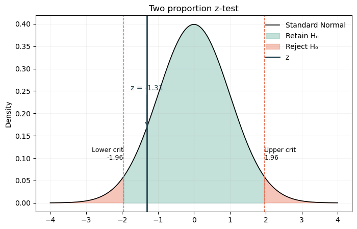
Two‑proportion z‑test: z = -1.3116, p = 0.189653
# Wald 95% CI for each proportion
ci_treat = proportion_confint(conv_treat, n_treat, method='normal')
ci_ctrl  = proportion_confint(conv_control, n_control, method='normal')

# Difference in proportions & CI (Wald)
p_hat_t = conv_treat / n_treat
p_hat_c = conv_control / n_control
diff = p_hat_t - p_hat_c
se = np.sqrt(p_hat_t*(1-p_hat_t)/n_treat + p_hat_c*(1-p_hat_c)/n_control)
ci_diff = (diff - 1.96*se, diff + 1.96*se)

print(f"Counts (treat/control): {conv_treat}/{n_treat} vs {conv_control}/{n_control}")
print(f"p_treat = {p_hat_t:.5f} 95% CI {ci_treat}")
print(f"p_ctrl  = {p_hat_c:.5f} 95% CI {ci_ctrl}")
print(f"Diff (treat - control) = {diff:.5f} 95% CI {ci_diff}")
Counts (treat/control): 17264/145311 vs 17489/145274
p_treat = 0.11881 95% CI (0.11714362162601945, 0.12047087417952866)
p_ctrl  = 0.12039 95% CI (0.11871294722381814, 0.12205966177710426)
Diff (treat - control) = -0.00158 95% CI (-0.003938713688889012, 0.0007806004935147211)
Decision rule: यदि p < 0.05, तो \(H_0\) को अस्वीकार करें और निष्कर्ष निकालें कि conversion pages के बीच भिन्न है। अन्यथा, \(H_0\) को अस्वीकार करने में असफल रहें।
चूंकि two-proportion z-test के लिए p=0.189 > 0.05 है, हम Null hypothesis को अस्वीकार करने में असफल हैं। इसका मतलब है कि नए और पुराने page के पास users को convert करने का लगभग समान मौका है। हम e-commerce कंपनी को पुराने page को बनाए रखने की सिफारिश करते हैं। इससे नए page बनाने में समय और पैसे की बचत होगी।
def plot_z_hypothesis(
    data_list,
    pop_mean=0.0,
    pop_sd=1.0,
    alternative='two.sided',   # 'two.sided' | 'greater' | 'less'
    type_test = 'mean', #'mean' | 'prob'
    alpha=0.05,
    label='Sampling distribution',
    title='z-test (sampling distribution of x̄)',
    x_label = "Sampling distribution of x̄",
    figsize=(8, 5)
):
    """
    Sampling distribution of sample mean के लिए z-test निर्णय क्षेत्रों का दृश्य।

    Parameters
    ----------
    data_list : array-like
        Sample values (used only to compute x̄ and n).
    pop_mean : float
        Hypothesized population mean (μ under H0).
    pop_sd : float
        Known population standard deviation (σ).
    alternative : str
        'two.sided', 'greater', or 'less' (same semantics as your R code).
    alpha : float
        Critical regions के लिए significance level.
    label : str
        Distribution curve के लिए label.
    title : str
        Plot title.
    figsize : tuple
        Figure size.

    Returns
    -------
    fig, ax : matplotlib Figure and Axes
    """
    x = np.asarray(data_list)
    n = len(x)
    xbar = np.mean(x)

    # Mean का standard error
    se = pop_sd / np.sqrt(n)

    # μ के चारों ओर ±4 SE के लिए plotting की सीमा (जैसे आपके R function में)
    grid = np.linspace(pop_mean - 4 * se, pop_mean + 4 * se, 4001)
    pdf = stats.norm.pdf(grid, loc=pop_mean, scale=se)

    # चुने गए alternative के लिए H0 के तहत critical cutoffs की गणना करें
    if alternative == 'two.sided':
        # symmetric cutoffs: (alpha/2) और (1 - alpha/2)
        lower_cut = stats.norm.ppf(alpha / 2, loc=pop_mean, scale=se)
        upper_cut = stats.norm.ppf(1 - alpha / 2, loc=pop_mean, scale=se)

        # Cutoffs के बीच बनाए रखें; बाहर अस्वीकार करें
        retain_mask = (grid >= lower_cut) & (grid <= upper_cut)
        reject_mask = ~retain_mask

    elif alternative == 'greater':
        # दाहिनी पूंछ पर अस्वीकार करें
        cutoff = stats.norm.ppf(1 - alpha, loc=pop_mean, scale=se)
        retain_mask = (grid <= cutoff)
        reject_mask = (grid > cutoff)
        lower_cut, upper_cut = None, cutoff

    elif alternative == 'less':
        # बाईं पूंछ पर अस्वीकार करें
        cutoff = stats.norm.ppf(alpha, loc=pop_mean, scale=se)
        retain_mask = (grid >= cutoff)
        reject_mask = (grid < cutoff)
        lower_cut, upper_cut = cutoff, None
    else:
        raise ValueError("alternative must be one of {'two.sided','greater','less'}")

    # सुविधा के लिए R pipeline की तरह एक DataFrame बनाएं (वैकल्पिक)
    df = pd.DataFrame({'x': grid, 'pdf': pdf, 'retain': retain_mask})

    # Plot
    fig, ax = plt.subplots(figsize=figsize)
    ax.plot(df['x'], df['pdf'], color='black', lw=1.2, label=label)

    # Retain क्षेत्र को छायांकित करें
    ax.fill_between(df['x'], 0, df['pdf'], where=df['retain'], color='#69b3a2', alpha=0.4, label='Retain H₀')

    # अस्वीकार क्षेत्र(s) को छायांकित करें
    ax.fill_between(df['x'], 0, df['pdf'], where=~df['retain'], color='#e76f51', alpha=0.4, label='Reject H₀')

    # Critical lines
    if alternative == 'two.sided':
        ax.axvline(lower_cut, color='#e76f51', ls='--', lw=1)
        ax.axvline(upper_cut, color='#e76f51', ls='--', lw=1)
        ax.text(lower_cut, ax.get_ylim()[1]*0.3, f"Lower crit\n{lower_cut:.2f}", ha='right', va='top', fontsize=9)
        ax.text(upper_cut, ax.get_ylim()[1]*0.3, f"Upper crit\n{upper_cut:.2f}", ha='left', va='top', fontsize=9)
    elif alternative == 'greater':
        ax.axvline(upper_cut, color='#e76f51', ls='--', lw=1)
        ax.text(upper_cut, ax.get_ylim()[1]*0.9, f"Crit\n{upper_cut:.2f}", ha='left', va='top', fontsize=9)
    elif alternative == 'less':
        ax.axvline(lower_cut, color='#e76f51', ls='--', lw=1)
        ax.text(lower_cut, ax.get_ylim()[1]*0.9, f"Crit\n{lower_cut:.2f}", ha='right', va='top', fontsize=9)

    # x̄ line और annotation
    if(type_test == 'prob'):
        ax.axvline(xbar, color='#264653', lw=2, ls='-', label='z')
        ax.annotate(f"z = {xbar:.2f}",
                xy=(xbar, stats.norm.pdf(xbar, loc=pop_mean, scale=se)),
                xytext=(xbar, ax.get_ylim()[1]*0.6),
                arrowprops=dict(arrowstyle='->', color='#264653'),
                ha='center', color='#264653')
    else:
        ax.axvline(xbar, color='#264653', lw=2, ls='-', label='Sample mean (x̄)')
        ax.annotate(f"x̄ = {xbar:.2f}",
                xy=(xbar, stats.norm.pdf(xbar, loc=pop_mean, scale=se)),
                xytext=(xbar, ax.get_ylim()[1]*0.6),
                arrowprops=dict(arrowstyle='->', color='#264653'),
                ha='center', color='#264653')

    ax.set_title(title)
    ax.set_xlabel(x_label)
    ax.set_ylabel("Density")
    ax.legend(loc='upper right', frameon=False)
    ax.grid(alpha=0.15)
    plt.show();
plot_z_hypothesis([z_stat], type_test = 'prob', title='Two proportion z-test', label = 'Standard Normal', x_label = '')
Welch’s t‑Test : Effect of Vitamin C on Tooth Growth
यह क्लासिक dataset Vitamin C के प्रभाव को गिनी पिग्स में tooth growth पर खोजता है, जो पोषण विज्ञान में एक मौलिक प्रयोग है। प्रतिक्रिया चर odontoblasts की लंबाई है, जो दांत के विकास के लिए जिम्मेदार कोशिकाएँ हैं। साठ गिनी पिग्स को दो वितरण विधियों में से एक में Vitamin C प्राप्त करने के लिए यादृच्छिक रूप से सौंपा गया:
1. Orange Juice (OJ)
2. Ascorbic Acid (VC) (Vitamin C का एक सिंथेटिक रूप)
प्रत्येक जानवर को तीन खुराक स्तरों में से एक दिया गया: 0.5 mg/day, 1 mg/day, या 2 mg/day। प्रयोग का उद्देश्य यह निर्धारित करना है कि क्या वितरण विधि tooth growth को प्रभावित करती है, खुराक को नियंत्रित करते हुए।
Why it matters:
विभिन्न Vitamin C स्रोतों की प्रभावशीलता को समझना आहार संबंधी सिफारिशों और पूरक फॉर्मूलेशन को मार्गदर्शित कर सकता है। आधुनिक विश्लेषण में, इस प्रकार का परीक्षण स्वास्थ्य देखभाल में दो उपचारों या हस्तक्षेपों की तुलना करने या उत्पाद डिजाइन में A/B परीक्षण के समान है।
Hypothesis:
\(H_0\): दोनों वितरण विधियों (OJ और VC) के लिए औसत tooth length समान है।
\(H_1\): दोनों विधियों के बीच औसत tooth length भिन्न है।
यह विश्लेषण 0.5 mg/day खुराक स्तर पर केंद्रित है; अन्य खुराक के लिए समान विश्लेषण किए जा सकते हैं।
Result Interpretation: Welch’s t-test चलाने के बाद, यदि p-value 0.05 से कम है, तो हम null hypothesis को अस्वीकार करते हैं, निष्कर्ष निकालते हैं कि वितरण विधि tooth growth को महत्वपूर्ण रूप से प्रभावित करती है। यदि p-value 0.05 से अधिक है, तो हम \(H_0\) को अस्वीकार करने में असफल रहते हैं, यह सुझाव देते हुए कि OJ और VC के बीच कोई मापने योग्य अंतर नहीं है। इसके अलावा, Cohen’s d की रिपोर्टिंग अंतर के आकार को मापने में मदद करती है, जो व्यावहारिक महत्व के लिए महत्वपूर्ण है।
Dataset: R ToothGrowth (OJ vs VC).
CSV: https://raw.githubusercontent.com/vincentarelbundock/Rdatasets/master/csv/datasets/ToothGrowth.csv
Variables: len (tooth length), supp ∈ {OJ, VC}.
Hypotheses (two‑sided):
- \(H_0: \mu_{\text{OJ}} = \mu_{ ext{VC}}\)
- \(H_1: \mu_{\text{OJ}}\neq \mu_{ ext{VC}}\)
Assumptions: Independent samples; normality (approx); Welch’s t‑test does not assume equal variance.
# Load ToothGrowth
url_tg = "https://raw.githubusercontent.com/vincentarelbundock/Rdatasets/master/csv/datasets/ToothGrowth.csv"
tg = pd.read_csv(url_tg)
# Drop the Rdatasets index column
for c in tg.columns:
    if 'Unnamed' in c:
        tg = tg.drop(columns=[c])
tg.head()
| rownames | len | supp | dose | |
|---|---|---|---|---|
| 0 | 1 | 4.200000 | VC | 0.500000 |
| 1 | 2 | 11.500000 | VC | 0.500000 |
| 2 | 3 | 7.300000 | VC | 0.500000 |
| 3 | 4 | 5.800000 | VC | 0.500000 |
| 4 | 5 | 6.400000 | VC | 0.500000 |
# Groups
oj = tg.loc[(tg['supp']=='OJ') & (tg.dose == 0.5),'len']
vc = tg.loc[(tg['supp']=='VC') & (tg.dose == 0.5),'len']

# Welch's t-test
t_stat, p_val = stats.ttest_ind(oj, vc, equal_var=False)

# Cohen's d (using pooled SD with group sizes)
def cohens_d(x, y):
    nx, ny = len(x), len(y)
    sx2, sy2 = np.var(x, ddof=1), np.var(y, ddof=1)
    sp2 = ((nx-1)*sx2 + (ny-1)*sy2) / (nx+ny-2)
    d = (np.mean(x) - np.mean(y)) / np.sqrt(sp2)
    return d

d = cohens_d(oj, vc)

print(f"Welch t‑test: t = {t_stat:.4f}, p = {p_val:.6f}")
print(f"Mean's: OJ = {np.mean(oj):.3f}, VC = {np.mean(vc):.3f}")
print(f"Cohen's d = {d:.3f}")
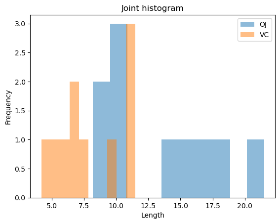
Welch t‑test: t = 3.1697, p = 0.006359
Mean's: OJ = 13.230, VC = 7.980
Cohen's d = 1.418
Decision rule: यदि p < 0.05, तो \(H_0\) को अस्वीकार करें → यह प्रमाण है कि वितरण विधि औसत tooth length को प्रभावित करती है। Cohen's d के मान 0.2 का मतलब है समूहों के बीच छोटा अंतर, 0.5 के लिए मध्यम, और 0.8 या उससे अधिक के लिए बड़े प्रभाव।
Result: OJ अधिक प्रभावी है: T-tests दिखाते हैं कि इन निम्न खुराकों पर दोनों वितरण विधियों के बीच सांख्यिकीय रूप से महत्वपूर्ण अंतर है, जिसमें orange juice अधिक tooth growth की ओर ले जाता है। P-values: P-values \(0.05\) से नीचे हैं, जो दर्शाता है कि अंतर यादृच्छिक अवसर के कारण होने की संभावना नहीं है। उदाहरण के लिए, 0.5mg पर, p-value लगभग \(0.006\) है।
def plot_bivariate_histograms(dataset, con_col, cat_col, title='', x_label = ''):
    bi_con_cat = dataset.groupby([cat_col])[con_col].plot.hist(alpha = 0.5)
    plt.xlabel(con_col)
    plt.legend(dataset.groupby([cat_col])[con_col].count().axes[0].tolist())
    plt.title(title)
    plt.xlabel(x_label)
    plt.show();
plot_bivariate_histograms(tg[tg.dose==0.5], 'len', 'supp', title='Joint histogram', x_label = 'Length')
One‑Way ANOVA : Branch‑wise Gross Income (with Tukey HSD)
यह dataset म्यांमार में एक सुपरमार्केट श्रृंखला से विस्तृत लेनदेन रिकॉर्ड कैप्चर करता है, जो तीन प्रमुख शहरों: यांगून, नायपीडॉ और मंडले को कवर करता है। डेटा जनवरी से मार्च 2019 तक तीन महीने की अवधि में फैला हुआ है, जो खुदरा संचालन का समृद्ध दृश्य प्रदान करता है। प्रत्येक रिकॉर्ड में शाखा स्थान, उत्पाद लाइन, ग्राहक जनसांख्यिकी, भुगतान विधियाँ, और वित्तीय मैट्रिक्स जैसे gross income और कुल बिक्री की जानकारी शामिल है।
हमारे hypothesis test के लिए, हम यह जांचने पर ध्यान केंद्रित करते हैं कि क्या शाखा स्थान gross income को प्रभावित करता है, जो लाभप्रदता के लिए एक महत्वपूर्ण मैट्रिक्स है। खुदरा प्रबंधकों को अक्सर यह जानने की आवश्यकता होती है कि क्या कुछ शाखाएँ लगातार अन्य से बेहतर प्रदर्शन करती हैं, क्योंकि यह जानकारी संसाधन आवंटन, विपणन रणनीतियों, और इन्वेंटरी योजना को मार्गदर्शित कर सकती है।
Hypothesis:
\(H_0\): सभी तीन शाखाओं (A, B, C) के लिए औसत gross income समान है।
\(H_1\): कम से कम एक शाखा का औसत gross income भिन्न है।
Why it matters: यदि परीक्षण महत्वपूर्ण अंतर प्रकट करता है, तो प्रबंधन अंतर्निहित कारकों की जांच कर सकता है जैसे ग्राहक खरीदने की शक्ति, शाखा का आकार, या स्थानीय विपणन की प्रभावशीलता। यह विश्लेषण वास्तविक दुनिया के व्यापार बुद्धिमत्ता कार्यों के समान है जहाँ data-driven निर्णय संचालन और लाभप्रदता को अनुकूलित करते हैं।
Result Interpretation: ANOVA चलाने के बाद, यदि p-value 0.05 से कम है, तो हम null hypothesis को अस्वीकार करते हैं, निष्कर्ष निकालते हैं कि शाखा स्थान gross income को प्रभावित करता है। Tukey HSD का उपयोग करके post-hoc विश्लेषण यह पहचानता है कि कौन सी शाखाएँ महत्वपूर्ण रूप से भिन्न हैं, जिससे सुधार के लिए लक्षित रणनीतियाँ सक्षम होती हैं।
Dataset: Supermarket Sales (तीन शाखाएँ: A, B, C).
CSV: https://raw.githubusercontent.com/selva86/datasets/master/supermarket_sales.csv
Outcome: gross income (continuous). Factor: Branch (A/B/C).
Hypotheses:
- \(H_0: \mu_A = \mu_B = \mu_C\)
- \(H_1\): कम से कम एक mean भिन्न है
Plan: ANOVA (ANalysis Of VAriance) को फिट करें, Levene का उपयोग करके homogeneity की जांच करें, फिर Tukey HSD के लिए post‑hoc pairwise comparisons करें।
# Load Supermarket Sales
df = pd.read_csv("https://raw.githubusercontent.com/selva86/datasets/master/supermarket_sales.csv")

# Tidy column names
df.columns = [c.strip().replace(' ', '_').lower() for c in df.columns]

df
| invoice_id | branch | city | customer_type | gender | product_line | unit_price | quantity | tax_5% | total | date | time | payment | cogs | gross_margin_percentage | gross_income | rating | |
|---|---|---|---|---|---|---|---|---|---|---|---|---|---|---|---|---|---|
| 0 | 750-67-8428 | A | Yangon | Member | Female | Health and beauty | 74.690000 | 7 | 26.141500 | 548.971500 | 1/5/2019 | 13:08 | Ewallet | 522.830000 | 4.761905 | 26.141500 | 9.100000 |
| 1 | 226-31-3081 | C | Naypyitaw | Normal | Female | Electronic accessories | 15.280000 | 5 | 3.820000 | 80.220000 | 3/8/2019 | 10:29 | Cash | 76.400000 | 4.761905 | 3.820000 | 9.600000 |
| 2 | 631-41-3108 | A | Yangon | Normal | Male | Home and lifestyle | 46.330000 | 7 | 16.215500 | 340.525500 | 3/3/2019 | 13:23 | Credit card | 324.310000 | 4.761905 | 16.215500 | 7.400000 |
| 3 | 123-19-1176 | A | Yangon | Member | Male | Health and beauty | 58.220000 | 8 | 23.288000 | 489.048000 | 1/27/2019 | 20:33 | Ewallet | 465.760000 | 4.761905 | 23.288000 | 8.400000 |
| 4 | 373-73-7910 | A | Yangon | Normal | Male | Sports and travel | 86.310000 | 7 | 30.208500 | 634.378500 | 2/8/2019 | 10:37 | Ewallet | 604.170000 | 4.761905 | 30.208500 | 5.300000 |
| ... | ... | ... | ... | ... | ... | ... | ... | ... | ... | ... | ... | ... | ... | ... | ... | ... | ... |
| 995 | 233-67-5758 | C | Naypyitaw | Normal | Male | Health and beauty | 40.350000 | 1 | 2.017500 | 42.367500 | 1/29/2019 | 13:46 | Ewallet | 40.350000 | 4.761905 | 2.017500 | 6.200000 |
| 996 | 303-96-2227 | B | Mandalay | Normal | Female | Home and lifestyle | 97.380000 | 10 | 48.690000 | 1,022.490000 | 3/2/2019 | 17:16 | Ewallet | 973.800000 | 4.761905 | 48.690000 | 4.400000 |
| 997 | 727-02-1313 | A | Yangon | Member | Male | Food and beverages | 31.840000 | 1 | 1.592000 | 33.432000 | 2/9/2019 | 13:22 | Cash | 31.840000 | 4.761905 | 1.592000 | 7.700000 |
| 998 | 347-56-2442 | A | Yangon | Normal | Male | Home and lifestyle | 65.820000 | 1 | 3.291000 | 69.111000 | 2/22/2019 | 15:33 | Cash | 65.820000 | 4.761905 | 3.291000 | 4.100000 |
| 999 | 849-09-3807 | A | Yangon | Member | Female | Fashion accessories | 88.340000 | 7 | 30.919000 | 649.299000 | 2/18/2019 | 13:28 | Cash | 618.380000 | 4.761905 | 30.919000 | 6.600000 |
1000 rows × 17 columns
# One-way ANOVA
model = ols('gross_income ~ C(branch)', data=df).fit()
anova_tbl = sm.stats.anova_lm(model, typ=2)
print(anova_tbl)
sum_sq df F PR(>F)
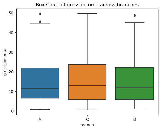
C(branch) 242.602644 2.000000 0.884583 0.413210
Residual 136,716.894906 997.000000 NaN NaN
# Levene test for homogeneity of variances
from scipy.stats import levene
branch_a = df[df['branch']=='A']['gross_income']
branch_b = df[df['branch']=='B']['gross_income']
branch_c = df[df['branch']=='C']['gross_income']
print("Levene p-value:", levene(branch_a, branch_b, branch_c).pvalue)
Levene p-value: 0.08946425577002974
# Tukey HSD post-hoc
tukey = pairwise_tukeyhsd(endog=df['gross_income'], groups=df['branch'], alpha=0.05)
print(tukey.summary())
Multiple Comparison of Means - Tukey HSD, FWER=0.05
===================================================
group1 group2 meandiff p-adj   lower  upper  reject
---------------------------------------------------
     A      B    0.358 0.9171 -1.7627 2.4788  False
     A      C   1.1784 0.3954 -0.9489 3.3057  False
     B      C   0.8203 0.6405 -1.3195 2.9602  False
---------------------------------------------------
Decision rule: यदि ANOVA p < 0.05, तो \(H_0\) को अस्वीकार करें और Tukey HSD का उपयोग करके भिन्न जोड़ों की पहचान करें। यदि Levene p < 0.05, तो Welch’s ANOVA या robust alternatives पर विचार करें।
चूंकि p=0.413 (PR(>F) = 0.413) 5% से अधिक है, हम Null hypothesis को अस्वीकार करने में असफल हैं और यह दावा कर सकते हैं कि तीनों शाखाओं की gross revenue समान है। इसके अतिरिक्त, हम देख सकते हैं कि variances homogeneous हैं (क्योंकि Levene का p-value > 5%) और प्रत्येक संयोजन के बीच t-tests कोई महत्व नहीं दिखाते हैं (Tukey का परीक्षण मूलतः एक t-test है, सिवाय इसके कि यह family-wise error rate के लिए सुधार करता है)।
bi_variate_boxplot = sns.boxplot(x="branch", y="gross_income", data=df)
bi_variate_boxplot.set(title = 'Box Chart of gross income across branches');
Chi‑Square Test of Independence: Gender × Product Category (Retail)
Multi‑category retail में, merchandising टीमें इस बात की गहरी चिंता करती हैं कि कौन क्या खरीदता है। यह वास्तविक ग्राहक खरीदारी dataset इस्तांबुल (2021–2023) में कई शॉपिंग मॉल में लेनदेन को कवर करता है और प्रत्येक खरीद के लिए लिंग और उत्पाद श्रेणी को शामिल करता है। हम यह परीक्षण करेंगे कि क्या उत्पाद श्रेणी की प्राथमिकताएँ लिंग के अनुसार भिन्न होती हैं, जो assortment planning, aisle placement, personalized recommendations, targeted promotions, और store layout निर्णयों को सूचित कर सकती हैं।
Variables:
- gender ∈ {Male, Female}
- category ∈ {जैसे, Clothing, Electronics, Accessories, …} (फाइल में कई श्रेणियाँ मौजूद हैं)
Hypotheses (Chi‑Square Test of Independence):
\(H_0\): Gender और product category स्वतंत्र हैं (कोई संबंध नहीं)।
\(H_1\): Gender और product category जुड़े हुए हैं (श्रेणी की प्राथमिकता लिंग पर निर्भर करती है)।
Why it matters:
एक महत्वपूर्ण संबंध यह सुझाव देता है कि लिंग के अनुसार श्रेणी की प्राथमिकताएँ भिन्न हैं। खुदरा विक्रेता प्रचार, सामग्री, इन्वेंटरी मिश्रण, और स्टोर प्रदर्शन को बेहतर ढंग से मांग के अनुसार समायोजित कर सकते हैं, जो अक्सर conversion rates और gross margin में सुधार करता है।
Assumptions & Data Checks:
- पर्याप्त अपेक्षित गणनाएँ (preferably ≥ 5 per cell)। यदि कुछ श्रेणियाँ दुर्लभ हैं, तो समान श्रेणियों को समूहित करने पर विचार करें या मानकों को संतुष्ट करने के लिए शीर्ष N श्रेणियों का विश्लेषण करें।
- अवलोकन स्वतंत्र हैं (प्रत्येक पंक्ति एक अलग लेनदेन है)।
(ये सभी मानक स्थितियाँ हैं जो Chi‑Square परीक्षण में श्रेणीबद्ध विश्लेषण के लिए होती हैं।)
Dataset Source:
Customer Shopping Data (GitHub) — file: customer_shopping_data.csv
Interpretation:
1. यदि p < 0.05, तो \(H_0\) को अस्वीकार करें: gender और product category जुड़े हुए हैं।
2. Cramér’s V संबंध की ताकत को इंगित करता है: ~0.1 = कमजोर, ~0.3 = मध्यम, ~0.5 = मजबूत।
हम Chi‑square independence परीक्षण और Cramér’s V को प्रभाव आकार के रूप में गणना करेंगे।
import pandas as pd
from scipy.stats import chi2_contingency
import numpy as np

# Load dataset
url = "https://raw.githubusercontent.com/gokcengiz/Shopping-data-analysis/main/customer_shopping_data.csv"
df = pd.read_csv(url)
df
| invoice_no | customer_id | gender | age | category | quantity | price | payment_method | invoice_date | shopping_mall | |
|---|---|---|---|---|---|---|---|---|---|---|
| 0 | I138884 | C241288 | Female | 28 | Clothing | 5 | 1,500.400000 | Credit Card | 5/8/2022 | Kanyon |
| 1 | I317333 | C111565 | Male | 21 | Shoes | 3 | 1,800.510000 | Debit Card | 12/12/2021 | Forum Istanbul |
| 2 | I127801 | C266599 | Male | 20 | Clothing | 1 | 300.080000 | Cash | 9/11/2021 | Metrocity |
| 3 | I173702 | C988172 | Female | 66 | Shoes | 5 | 3,000.850000 | Credit Card | 16/05/2021 | Metropol AVM |
| 4 | I337046 | C189076 | Female | 53 | Books | 4 | 60.600000 | Cash | 24/10/2021 | Kanyon |
| ... | ... | ... | ... | ... | ... | ... | ... | ... | ... | ... |
| 99452 | I219422 | C441542 | Female | 45 | Souvenir | 5 | 58.650000 | Credit Card | 21/09/2022 | Kanyon |
| 99453 | I325143 | C569580 | Male | 27 | Food & Beverage | 2 | 10.460000 | Cash | 22/09/2021 | Forum Istanbul |
| 99454 | I824010 | C103292 | Male | 63 | Food & Beverage | 2 | 10.460000 | Debit Card | 28/03/2021 | Metrocity |
| 99455 | I702964 | C800631 | Male | 56 | Technology | 4 | 4,200.000000 | Cash | 16/03/2021 | Istinye Park |
| 99456 | I232867 | C273973 | Female | 36 | Souvenir | 3 | 35.190000 | Credit Card | 15/10/2022 | Mall of Istanbul |
99457 rows × 10 columns
# Build contingency table: Gender vs Payment Method
ct = pd.crosstab(df['category'], df['gender'])
chi2, p, dof, expected = chi2_contingency(ct)
print("Contingency Table:\n", ct)
print(f"Chi-square = {chi2:.4f}, p-value = {p:.6f}, dof = {dof}")
Contingency Table:
gender Female Male
category
Books 2906 2075
Clothing 20652 13835
Cosmetics 9070 6027
Food & Beverage 8804 5972
Shoes 5967 4067
Souvenir 3017 1982
Technology 2981 2015
Toys 6085 4002
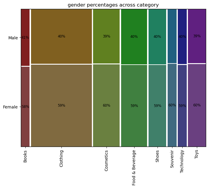
Chi-square = 7.5679, p-value = 0.372234, dof = 7
p value 0.37 > 0.05 यह दर्शाता है कि हम Null Hypothesis को अस्वीकार करने में असफल हैं। श्रेणी के संबंध में लिंग के बीच कोई अंतर नहीं है।
# Compute Cramér's V
n = ct.values.sum()
phi2 = chi2 / n
r, c = ct.shape
cramers_v = np.sqrt(phi2 / min(r-1, c-1))

print(f"Cramér's V = {cramers_v:.3f}")
Cramér's V = 0.009
0.009 एक बहुत कमजोर संबंध को दर्शाता है
from statsmodels.graphics.mosaicplot import mosaic
def plot_mosaics(data, x_col, y_col, title='', colors_list =[]):
    dict_of_tuples = {}

    # प्रतिशत को प्रिंट करने के लिए साफ सेट बनाएं
    for x_col_ in data[x_col].unique():
        for y_col_ in data[y_col].unique():
            n = len(data[(data[x_col]==x_col_)&(data[y_col]==y_col_)][x_col])
            d = len(data[(data[x_col]==x_col_)][x_col])
            len_ = len(data[x_col])
            if((d==0) or (n/d<=0.04)):
                # यदि किसी श्रेणी के भीतर प्रतिशत 4% से कम है, तो प्रतिशत प्रिंट न करें
                dict_of_tuples[(str(x_col_), str(y_col_))] = ''
            elif(n/len_<=0.02):
                # यदि इसका एक छोटा वर्ग है जिसमें कुल डेटा का 2% से कम है, तो विश्लेषण न करें
                dict_of_tuples[(str(x_col_), str(y_col_))] = ''
            else:
                dict_of_tuples[(str(x_col_), str(y_col_))] = str(int(n/d*100))+"%"

    dict_of_colors = dict_of_tuples.copy()
    if(len(colors_list)>0):
        # रंगों का एक साफ सेट बनाएं
        for i, x_col_ in enumerate(data[x_col].unique()):
            for y_col_ in data[y_col].unique():
                dict_of_colors[(str(x_col_), str(y_col_))] = {'color':colors_list[i], 'alpha':0.8}

    # Mosaic plot को प्लॉट करें
    labelizer = lambda k: dict_of_tuples[k]
    fig, ax = plt.subplots(figsize=(8,6))
    if(len(colors_list)>0):
        mosaic(data.sort_values([x_col, y_col]), [x_col, y_col],
               statistic = False, axes_label = True, label_rotation = [90, 0],
               labelizer=labelizer, properties=dict_of_colors, gap=0.008, ax=ax)
    else:
        mosaic(data.sort_values([x_col, y_col]), [x_col, y_col],
               statistic = False, axes_label = True, label_rotation = [90, 0],
               labelizer=labelizer, gap=0.008, ax=ax)
    if(title==''):
        plt.title(str(y_col) + ' percentages across ' + str(x_col))
    else:
        plt.title(title)
    plt.show();
plot_mosaics(df, 'category', 'gender')
Decision rule: यदि p < 0.05, तो \(H_0\) को अस्वीकार करें। संबंध की ताकत को मापने के लिए Cramér’s V की रिपोर्ट करें।
चूंकि p 5% से अधिक है, हम null hypothesis को अस्वीकार करने में असफल हैं, जो लिंग और उत्पाद श्रेणी के बीच कोई महत्वपूर्ण संबंध नहीं दर्शाता है।
References
- Udacity A/B test (ab_data.csv) GitHub mirror: https://github.com/beery4010/Analyze-AB-Test-Results
- ToothGrowth dataset (Rdatasets CSV): https://github.com/vincentarelbundock/Rdatasets/blob/master/csv/datasets/ToothGrowth.csv
- Supermarket Sales dataset (selva86/datasets CSV): https://github.com/selva86/datasets/blob/master/supermarket_sales.csv
- Retail data : https://github.com/gokcengiz/Shopping-data-analysis