Introduction to stationarity (R)
Time Series
A time series is a series of data points captured in time order. Most commonly, a time series is a sequence taken at successive equally spaced points in time. This post is the first in a series of blogs on time series methods and forecasting.
In this blog, we will discuss stationarity, random walk, deterministic drift and other vocabulary which form as foundation to time series:
Stochastic processes
A random or stochastic process is a collection of random variables ordered in time. It is denoted as \(Y_t\). For example, in-time of an employee is a stochastic process. How is in-time a stochastic process? Consider the in-time on a particular day is 9:00 AM. In theory, the in-time could be any particular value which depends on many factors like traffic, work load, weather etc. The figure 9:00 AM is a particular realization of many such possibilities. Therefore, we can say that in-time is a stochastic process whereas the actual values observed are a particular realization (sample) of the process.
Stationary Processes
A stochastic process is said to be stationary if the following conditions are met:
1. Mean is constant over time
2. Variance is constant over time
3. Value of the co-variance between two time periods depends only on the distance or gap or lag between the two time periods and not the actual time at which the co variance is computed
This type of process is also called weakly stationary, or co variance stationary, or second-order stationary or wide sense stationary process.
Written mathematically, the conditions are: $$ Mean: E(Y_t) = \mu $$ $$ Variance: var(Y_t) = E(Y_t-\mu)^2 = \sigma^2 $$ $$ Covariance: \gamma_k = E[(Y_y - \mu)(Y_{t+k} - \mu)] $$
Purely random or white noise process
A stochastic process is purely random if it has zero mean, constant variance, and is serially uncorrelated. An example of white noise is the error term in a linear regression which has zero mean, constant standard deviation and no auto-correlation.
Simulation
For simulating a stationary process, I am creating 100 realizations(samples) and comparing their mean, variance and co-variance. The data for 6 days and 5 realizations is shown:
| date | realization_1 | realization_2 | realization_25 | realization_50 | realization_100 | |
|---|---|---|---|---|---|---|
| 1 | 2021-12-28 | 0.3409607 | 0.5713826 | 0.2313986 | 0.6050719 | 0.5335372 |
| 2 | 2021-12-29 | 0.5554507 | 0.5244803 | 0.4288635 | 0.9073932 | 0.6350137 |
| 3 | 2021-12-30 | 0.1281935 | 0.1139629 | 0.2330727 | 0.8417148 | 0.8781020 |
| 10 | 2022-01-06 | 0.1901487 | 0.7607555 | 0.5620072 | 0.2611821 | 0.4575932 |
| 15 | 2022-01-11 | 0.8317412 | 0.6043582 | 0.0995929 | 0.9609510 | 0.2208680 |
| 30 | 2022-01-26 | 0.3612965 | 0.5961108 | 0.5965198 | 0.3048035 | 0.7668487 |
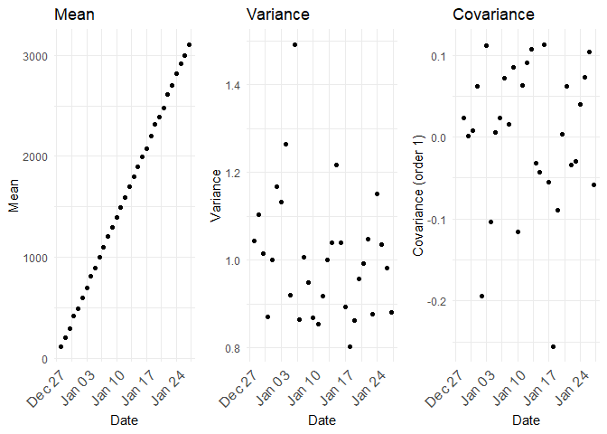
The mean, variance and co-variance between the samples (realizations) across are as follows:
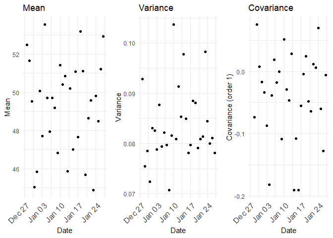
For a stationary process, the mean, variance and co variance are constant.
Non-stationary Processes
If a time series is not stationary, it is called a non-stationary time series. In other words, a non-stationary time series will have a time-varying mean or a time-varying variance or both. Random walk, random walk with drift etc are examples of non-stationary processes.
Random walk
Suppose \(\epsilon_t\) is a white noise error term with mean 0 and variance \(σ_2\). Then the series \(Y_t\) is said to be a random walk if $$ Y_t = Y_{t−1} + \epsilon_t $$ In the random walk model, the value of Y at time t is equal to its value at time (t − 1) plus a random shock.
For a random walk, $$ Y_1 = Y_0 + \epsilon_1 $$ $$ Y_2 = Y_1 + \epsilon_2 = Y_0 + \epsilon_1 + \epsilon_2 $$ $$ Y_3 = Y_2 + \epsilon_3 = Y_0 + \epsilon_1 + \epsilon_2 + \epsilon_3 $$ and so on.. In general we could write
$$ Y_t = Y_0 + \sum \epsilon_t $$ As $$ E(Y_t) = E(Y_0 + \sum \epsilon_t) = Y_0 $$ $$ var(Y_t) = t\times \sigma^2 $$
Although the mean is constant with time, the variance is proportional to time.
For simulating a random walk process, I am creating 100 realizations(samples) and comparing their mean, variance and co-variance. The data for 6 days of 5 realizations (samples) is shown:
| date | realization_1 | realization_2 | realization_25 | realization_50 | realization_100 | |
|---|---|---|---|---|---|---|
| 1 | 2021-12-28 | 4.000000 | 4.0000000 | 4.000000 | 4.000000 | 4.000000 |
| 2 | 2021-12-29 | 3.215170 | 4.9727559 | 4.981838 | 2.677480 | 4.209128 |
| 3 | 2021-12-30 | 2.400451 | 4.2477385 | 6.266374 | 3.249609 | 5.545876 |
| 10 | 2022-01-06 | 2.510370 | 4.1251187 | 8.500313 | 4.559066 | 7.634846 |
| 15 | 2022-01-11 | 6.286410 | 5.3430478 | 9.441353 | 2.147137 | 7.098887 |
| 30 | 2022-01-26 | 2.985008 | 0.2757552 | 5.219005 | 3.402089 | 4.125985 |
The mean, variance and covariances between the samples (realizations) across time would look like follows:
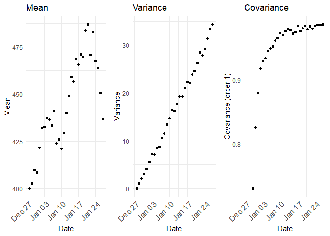
From the above plot, the mean of Y is equal to its initial, or starting value, which is constant, but as t increases, its variance increases indefinitely, thus violating a condition of stationarity.
A random walk process is also called as a unit root process.
Random walk with drift
If the random walk model predicts that the value at time t will equal the last period's value plus a constant, or drift (\(\delta\)), and a white noise term (\(ε_t\)), then the process is random walk with a drift.
$$ Y_t = \delta + Y_{t−1} + \epsilon_t $$ The mean $$ E(Y_t) = E(Y_0 + \sum \epsilon_t + \delta) = Y_0 + t\times\delta $$ so mean is dependent on time
and the variance $$ var(Y_t) = t\times \sigma^2 $$ is also dependent on time. As random walk with drift violates the conditions of stationary process, it is a non-stationary process.
| date | realization_1 | realization_2 | realization_25 | realization_50 | realization_100 | |
|---|---|---|---|---|---|---|
| 1 | 2021-12-28 | 4.000000 | 4.000000 | 4.000000 | 4.000000 | 4.000000 |
| 2 | 2021-12-29 | 6.707957 | 4.783724 | 5.082320 | 4.050322 | 6.047140 |
| 3 | 2021-12-30 | 6.154817 | 6.034937 | 6.593877 | 5.690097 | 6.443667 |
| 10 | 2022-01-06 | 3.092089 | 13.488318 | 13.143434 | 11.613472 | 8.216818 |
| 15 | 2022-01-11 | 4.827608 | 16.137101 | 12.706459 | 14.614712 | 12.535962 |
| 30 | 2022-01-26 | 8.567962 | 19.017960 | 20.586592 | 19.409629 | 14.157457 |
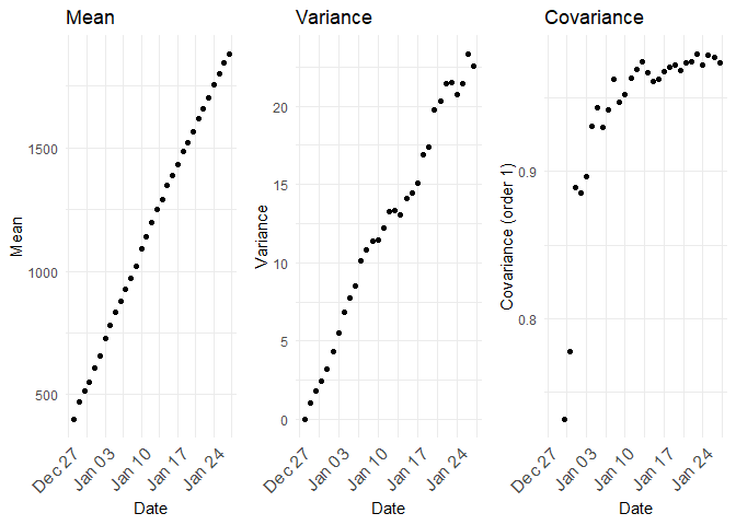
The mean, variance and the co-variance are all dependent on time.
Unit root stochastic process
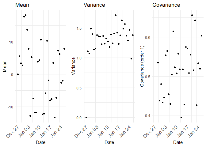
Unit root stochastic process is another name for Random walk process. A random walk process can be written as $$ Y_t = \rho \times Y_{t−1} + \epsilon_t $$ Where \(\rho = 1\). If \(|\rho| < 1\) then the process represents Markov first order auto regressive model which is stationary. Only for \(\rho = 1\) we get non-stationary. The distribution of mean, variance and co-variance for \(\rho =0.5\) is
Deterministic trend process
In the above random walk and random walk with drift, the trend component is stochastic in nature. If instead the trend is deterministic in nature, it will follow a deterministic trend process. $$ Y_t = β_1 + β_2\times t + \epsilon_t$$ In a deterministic trend process, the mean is \(β_1 + β_2\times t\) which is proportional with time, but the variance is constant. This type of process is also called as trend seasonality as subtracting mean of \(Y_t\) from \(Y_t\) will give us a stationary process. This procedure is called de-trending.
| date | realization_1 | realization_2 | realization_25 | realization_50 | realization_100 | |
|---|---|---|---|---|---|---|
| 1 | 2021-12-28 | 0.2435772 | 0.266316 | 1.634834 | 1.501271 | -0.2332093 |
| 2 | 2021-12-29 | 1.7185437 | 1.974812 | 1.128986 | 2.605209 | 1.0183324 |
| 3 | 2021-12-30 | 3.0196971 | 2.321355 | 3.529886 | 3.100916 | 3.2666808 |
| 10 | 2022-01-06 | 11.8821817 | 9.759775 | 11.575552 | 9.727393 | 9.3407779 |
| 15 | 2022-01-11 | 13.3588365 | 15.525071 | 15.037742 | 15.931198 | 14.2090916 |
| 30 | 2022-01-26 | 30.2218724 | 30.342918 | 30.405570 | 29.090780 | 29.6063424 |
A combination of deterministic and stochastic trend could also exist in a process.
Comparison.
A comparison of all the processes is shown below: 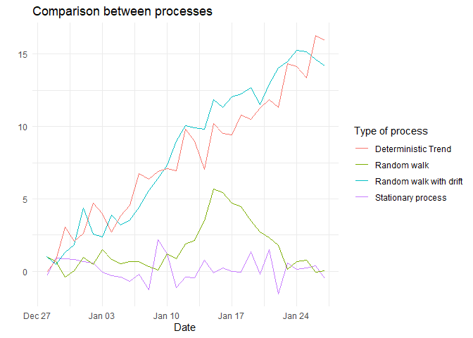
References
- Basic Econometrics - Damodar N Gujarati (textbook for reference)
- Business Analytics: The Science of Data-Driven Decision Making - Dinesh Kumar (textbook for reference)
- Customer Analytics at Flipkart.com - Naveen Bhansali (case study in Harvard Business Review)