Part and partial correlation
Introduction
The concept of partial correlation and part correlation plays an important role in regression model building. I always had a confusion between the two. In this post, I would like to explore the difference between the two and understand how and where they are used.
The data and the problem statement along with explanation of the different kinds of correlation coefficients can be found from the textbook Business Analytics: The Science of Data-Driven Decision Making. This post is largely inspired from the Example problem 10.1 found in Multiple linear regression chapter in the book.
The cumulative television ratings(CTRP), money spent on promotions(P) and advertisement revenue for 38 different television programmed are given in the data.
## # A tibble: 5 x 3
##    CTRP      P       R
##   <dbl>  <dbl>   <dbl>
## 1   117 172800 1457400
## 2   154 108000 1295100
## 3   115 176400 1207488
## 4   149 147600 1407444
## 5   118 169200 1272012
The summary statistics for the data is:
##       CTRP             P                R
##  Min.   : 90.0   Min.   : 75600   Min.   : 904776
##  1st Qu.:117.2   1st Qu.:108000   1st Qu.:1106700
##  Median :128.0   Median :126000   Median :1202532
##  Mean   :125.8   Mean   :131779   Mean   :1200763
##  3rd Qu.:136.0   3rd Qu.:150300   3rd Qu.:1294809
##  Max.   :156.0   Max.   :208800   Max.   :1457400
There are two factors that explain R, namely P and CTRP. I want to see individually how much they will be able to explain the total variance in \(y\). The total proportion of the variation in \(y\) explained by \(x\) is given by R square value of the regression. The R square and \(\beta\) values for both the independent variables when taken individually are as follows:
##
## Call:
## lm(formula = .outcome ~ ., data = dat)
##
## Residuals:
##     Min      1Q  Median      3Q     Max
## -229572  -80536   -3601   67967  297182
##
## Coefficients:
##             Estimate Std. Error t value Pr(>|t|)
## (Intercept)   621672     141428   4.396 0.000127 ***
## CTRP            4603       1113   4.135 0.000263 ***
## ---
## Signif. codes:  0 '***' 0.001 '**' 0.01 '*' 0.05 '.' 0.1 ' ' 1
##
## Residual standard error: 113300 on 30 degrees of freedom
## Multiple R-squared:  0.3631, Adjusted R-squared:  0.3418
## F-statistic:  17.1 on 1 and 30 DF,  p-value: 0.0002629
##
## [1] "----------------------------------------------------------------------------------------------------"
##
## Call:
## lm(formula = .outcome ~ ., data = dat)
##
## Residuals:
##     Min      1Q  Median      3Q     Max
## -218735  -88210   12298   63999  185209
##
## Coefficients:
##              Estimate Std. Error t value Pr(>|t|)
## (Intercept) 8.774e+05  8.247e+04   10.64 1.06e-11 ***
## P           2.527e+00  6.208e-01    4.07 0.000315 ***
## ---
## Signif. codes:  0 '***' 0.001 '**' 0.01 '*' 0.05 '.' 0.1 ' ' 1
##
## Residual standard error: 107600 on 30 degrees of freedom
## Multiple R-squared:  0.3558, Adjusted R-squared:  0.3343
## F-statistic: 16.57 on 1 and 30 DF,  p-value: 0.0003146
##
## [1] "----------------------------------------------------------------------------------------------------"
The outcome is as follows: For CTRP $$ Y = 677674 + 4175CTRP + \epsilon_{CTRP} \qquad Eq(1) $$ where \(\epsilon_{CTRP}\) is the unexplained error due to CTRP.
Similarly, for P, $$ Y = 87740 + 2.527P + \epsilon_{P} \qquad Eq(2) $$ where \(\epsilon_{P}\) is the unexplained error due to P
From the above outcome, I observe the following:
1. The total proportion of variation in \(y\) explained by CTRP and P individually are 28.15% and 35.58% respectively. (From R-square in the above results)
2. The \(\beta\) coefficients of CTRP and P are 4175 and 2.527 respectively. That means for every unit change in CTRP, the revenue increases by 4175 units while for every change in P the revenue increases by 2.527 units.
If both CTRP and P are independent, then I would think that if I tried to use both the variables in the model, then
1. The total explainable variation in \(y\) should be 28.15 + 35.58 = 63.73%. That means the model's R square should be 0.6373
2. The \(\beta\) coefficients should be same as before
Let's build a regression model using both these variables. In this model, the \(y\) variable (Revenue R) is explained using P (promotions) and CTRP. The output is shown below.
##
## Call:
## lm(formula = .outcome ~ ., data = dat)
##
## Residuals:
##     Min      1Q  Median      3Q     Max
## -125839  -25848    5388   26146  180440
##
## Coefficients:
##              Estimate Std. Error t value Pr(>|t|)
## (Intercept) 4.101e+04  9.096e+04   0.451    0.655
## CTRP        5.932e+03  5.766e+02  10.287 4.02e-12 ***
## P           3.136e+00  3.032e-01  10.344 3.47e-12 ***
## ---
## Signif. codes:  0 '***' 0.001 '**' 0.01 '*' 0.05 '.' 0.1 ' ' 1
##
## Residual standard error: 57550 on 35 degrees of freedom
## Multiple R-squared:  0.8319, Adjusted R-squared:  0.8223
## F-statistic: 86.62 on 2 and 35 DF,  p-value: 2.793e-14
The outcome is as follows: $$ Y = 41018 + 5932CTRP + 3.136P + \epsilon \qquad Eq(3) $$ where \(\epsilon\) is the unexplained error.
The total R-squared is 0.8319 which means that the total proportion of variation in \(y\) explained is 83.19%. We were expecting a r-squared of 0.6373. Even the \(\beta\) of CTRP is 5932 which was 4175 before. That means that for every one unit change in CTRP, 5932 units of Revenue will change (keeping P constant), instead of 4175 as we thought before.
So what is happening here?
Consider the following Venn diagram:
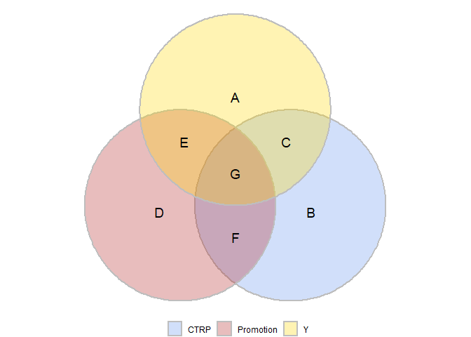
In the above diagram, the gold color is Y while the cornflower blue is CTRP and firebrick is Promotion. The area in circles show the variation in the variables. The intersection of 2 circles shows the variation explained in one variable by another variable.
I want to understand two things.
1. The increase in R squared due to addition of a variable. Assuming that the variable P already exists in the model, I would like to see how adding CTRP will change the R square value
2. How do I get the \(\beta\) value of CTRP in the combined model (Equation 3). The \(\beta_{CTRP}\) is nothing but the change when all other variables are kept constant, in this case when promotion is kept constant
Part or semi partial correlation
Part of semi partial correlation explains how much additional variation is explained by including a new parameter. If Promotion was already existing in the model, and I introduce CTRP, the variance explained by CTRP alone would be C/(A+E+G+C).
To get the same I should remove the 'G' part in the above diagram. That can be achieved by removing the influence of promotion in CTRP and then doing a regression of the remaining part (B + C) with \(y\).
The correlation coefficient when effect of other variables are removed from \(x\) but not from \(y\) is called as semi partial or part correlation coefficient.
The result of regression promotion with CTRP is as follows:
##
## Call:
## lm(formula = .outcome ~ ., data = dat)
##
## Residuals:
##     Min      1Q  Median      3Q     Max
## -39.131  -6.563   0.545   7.558  26.869
##
## Coefficients:
##               Estimate Std. Error t value Pr(>|t|)
## (Intercept)  1.417e+02  1.156e+01  12.253 2.09e-14 ***
## P           -1.201e-04  8.532e-05  -1.408    0.168
## ---
## Signif. codes:  0 '***' 0.001 '**' 0.01 '*' 0.05 '.' 0.1 ' ' 1
##
## Residual standard error: 16.63 on 36 degrees of freedom
## Multiple R-squared:  0.05219,    Adjusted R-squared:  0.02586
## F-statistic: 1.982 on 1 and 36 DF,  p-value: 0.1677
$$ CTRP = 141.7 -0.0001P + \epsilon_{P-CTRP} \qquad Eq(4)$$ Where \(\epsilon_{P-CTRP}\) is the unexplained error in CTRP due to P (B and C part).
The regression R-square of the unexplained error in CTRP with Y should give me the variation explained because of CTRP only.
##
## Call:
## lm(formula = .outcome ~ ., data = dat)
##
## Residuals:
##     Min      1Q  Median      3Q     Max
## -218369  -66614  -11444   61728  279858
##
## Coefficients:
##              Estimate Std. Error t value Pr(>|t|)
## (Intercept) 1200762.6    15746.4  76.256  < 2e-16 ***
## e_ctrp_p       5931.9      972.6   6.099 5.13e-07 ***
## ---
## Signif. codes:  0 '***' 0.001 '**' 0.01 '*' 0.05 '.' 0.1 ' ' 1
##
## Residual standard error: 97070 on 36 degrees of freedom
## Multiple R-squared:  0.5082, Adjusted R-squared:  0.4945
## F-statistic:  37.2 on 1 and 36 DF,  p-value: 5.126e-07
$$ Y = 1200762.6 +5931.9\epsilon_{P-CTRP} + \epsilon \qquad Eq(5)$$ where \(\epsilon\) is the unexplained error in Y due to CTRP alone (G, E and A part).
From here I can infer that an additional 50% of the variation in y is explained by adding CTRP variable. This is called as the semi partial or part correlation. The sum of r-squared when p alone is present in the model (variation explained in y due to P (Equation 2) ie: E and G part in the Venn diagram) and the part correlation R-squared when CTRP is added in the model (variation explained only by CTRP removing P ie: C part in Venn diagram) is close to the total R-Squared when both the variables are present in the model(equation 3).
Partial correlation
I want to understand how much Revenue changes with CTRP keeping Promotions constant (\(\beta_{CTRP}\) in Equation 3), to do this, I should remove the effect of P from both Y(revenue) and promotion. The correlation coefficient I get from removing the effect of all other variables in both \(y\) and \(x\) is called partial correlation coefficient. In the above Venn diagram, it is C/(C+A)
##
## Call:
## lm(formula = .outcome ~ ., data = dat)
##
## Residuals:
##     Min      1Q  Median      3Q     Max
## -125839  -25848    5388   26146  180440
##
## Coefficients:
##              Estimate Std. Error t value Pr(>|t|)
## (Intercept) 2.067e-10  9.205e+03    0.00        1
## e_ctrp_p    5.932e+03  5.686e+02   10.43 1.98e-12 ***
## ---
## Signif. codes:  0 '***' 0.001 '**' 0.01 '*' 0.05 '.' 0.1 ' ' 1
##
## Residual standard error: 56740 on 36 degrees of freedom
## Multiple R-squared:  0.7515, Adjusted R-squared:  0.7446
## F-statistic: 108.9 on 1 and 36 DF,  p-value: 1.977e-12
References
- Kumar, U. Dinesh. Business Analytics: The Science of Data-driven Decision Making. Wiley India, 2017.
- Cohen, Patricia, Stephen G. West, and Leona S. Aiken. Applied multiple regression/correlation analysis for the behavioral sciences. Psychology Press, 2014. (and related notes)
- Venn diagrams in R from scriptsandstatistics.wordpress.com
i. In this example the values are not exactly equal to each other because of suppressor variable