Multicollinearity (R)
I want to go through some basic statistical concepts before starting with the problem. I want to explain what is multicollinearity and how and when to tackle it.
Collinearity
Collinearity is a linear association between two variables. Two variables are perfectly collinear if there is an exact linear relationship between them. For example, \({\displaystyle X_{1}}\) and \({\displaystyle X_{2}}\) are perfectly collinear if there exist parameters \({\displaystyle \lambda _{0}}\) and \({\displaystyle \lambda _{1}}\) such that, for all observations i, we have
$$ X_{2i} = \lambda_0 + \lambda_1 X_{1i} $$ Here \({\displaystyle \lambda _{1}}\) can be considered as the slope of the equation and \({\displaystyle \lambda _{0}}\) is the intercept.
Correlation
Correlation is a numerical measure. It measures how close two variables are having a linear relationship with each other. The most popular form of correlation coefficient is the Pearson's coefficient(\(r_{xy}\)).
Pearson's product-moment coefficient
It is obtained by dividing the co-variance of the two variables by the product of their standard deviations.
\({\displaystyle r_{xy}=\mathrm {corr} (X,Y)={\mathrm {cov} (X,Y) \over \sigma _{X}\sigma _{Y}} = {\frac {\sum \limits _{i=1}^{n}(x_{i}-{\bar {x}})(y_{i}-{\bar {y}})}{(n-1)s_{x}s_{y}}}={\frac {\sum \limits _{i=1}^{n}(x_{i}-{\bar {x}})(y_{i}-{\bar {y}})}{\sqrt {\sum \limits _{i=1}^{n}(x_{i}-{\bar {x}})^{2}\sum \limits _{i=1}^{n}(y_{i}-{\bar {y}})^{2}}}},}\)
Where x and y are the means of X and Y, and \(s_{x}, s_{y}\) are the standard deviations of X and Y.
The Pearson correlation is \(+1\) in case of a perfect direct(increasing) linear relationship (correlation), \(-1\) in the case of a perfect decreasing (inverse) linear relationship(anti-correlation), and some value in the open interval \((-1, +1)\) in all other cases, indicating the degree of linear dependence between the variables. As it approaches zero there is less of a relationship(closer to uncorrelated). The closer the coefficient is to either \(-1\) or \(+1\), the stronger is the correlation between the variables.
If the variables are independent, Pearson's correlation coefficient is 0, but the converse is not true because the correlation coefficient detects only linear dependencies between two variables. For example, suppose the random variable X is symmetrically distributed about zero, and \(Y = X^{2}\). Then Y is completely determined by X, so that X and Y are perfectly dependent, but their correlation is zero.
Multicollinearity
Multicollinearity occurs when independent variables in a regression model are correlated. This correlation is a problem because independent variables should be independent. If the degree of correlation between variables is high, it can cause problems when I fit the model and interpret the results.
A key goal of regression (or classification) analysis is to isolate the relationship between each independent variable and the dependent variable. The interpretation of a regression coefficient is that it represents the mean change in the dependent variable for each 1 unit change in an independent variable when I hold all the other independent variables constant. That last portion is crucial for our discussion about multicollinearity.
The idea is that I can change the value of one independent variable and not the others. However, when independent variables are correlated, it indicates that changes in one variable are associated with shifts in another variable. The stronger the correlation, the more difficult it is to change one variable without changing another. It becomes difficult for the model to estimate the relationship between each independent variable and the dependent variable independently because the independent variables tend to change in unison.
What problems do multicollinearity cause?
- The coefficients become very sensitive to small changes in the model.
- I will not be able to trust the p-values to identify independent variables that are statistically significant.
That said, I need not always fix multicollinearity. Multicollinearity affects the coefficients and p-values, but it does not influence the predictions, precision of the predictions, and the goodness-of-fit statistics. If my primary goal is to make predictions, and I don't need to understand the role of each independent variable, I don't need to reduce severe multicollinearity.
In-time analysis problem
Now that I have discussed this much, let me continue with the in-time analysis problem. I want to analyse my entry time at office and understand how different factors effect it.
Collinearity checks are done after Univariate and multivariate analysis in EDA. One reason for doing so is that now I know how each factor looks like, and as collinearity is only a linear association between two explanatory variables, we can convert our factors to linear after applying some functions on them(log, square root etc).
After multivariate analysis, I currently have the factors
1. date (month / week day / season etc)
2. main_activity (means of transport)
3. hours.worked (of the previous day)
4. travelling.time (time it took to travel from house to office)
5. home.addr (the place of residence)
6. diff.out.time (previous day out of office time)
Out of these factors, only travelling.time, hours.worked and diff.out.time are continuous variables, so for now I will restrict my analysis to these three factors.
The dependent variable is diff.in.time (difference between my actual in time vs policy in-time)
| diff.in.time | date | main_activity | hours.worked | travelling.time | home.addr | diff.out.time |
|---|---|---|---|---|---|---|
| -14 | 2018-10-09 | ON_BICYCLE | 10.033333 | 1147.000 | New House | 76 |
| 35 | 2018-03-30 | IN_VEHICLE | 9.383333 | 854.006 | Old House | -12 |
| 31 | 2018-11-02 | ON_FOOT | 10.800000 | 2183.856 | New House | 77 |
| 1 | 2018-08-03 | IN_VEHICLE | 9.816667 | 633.513 | Old House | 48 |
| 22 | 2018-04-04 | IN_VEHICLE | 9.266667 | 1115.000 | Old House | -6 |
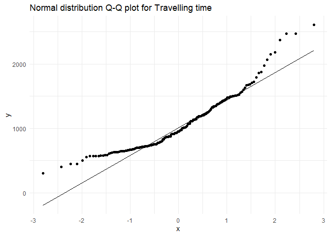
As a recap on univariate analysis, hours.worked and diff.in.out.time were exponential distributions(while checking for collinearity we should take their log for linear relationships),
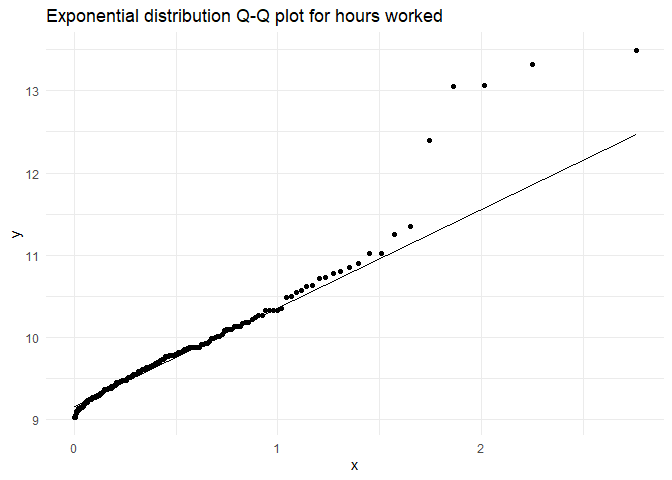
while travelling.time is close to a normal distribution(with an exponential tails, but let us ignore that for a now)
Testing for collinearity
One of the most popular tests to check multicollinearity is VIF factor(which will be discussed and calculated in linear regression blog post). What I want to instead do is visually see how the independent factors influence one another. I can do it in two main ways:
Correlation matrix
A correlation matrix is a table showing correlation coefficients(\(r_{xy}\)) between variables. Each cell in the table shows the correlation between two variables.
First I will make a reusable correlation matrix plotting function.
corr_matrix_plotting_fxn <- function(df){
  library(reshape)
  library(ggplot2)

  # Making a correlation matrix
  cormat <- round(cor(df), 2)

  # Getting the upper triangular matrix
  cormat[upper.tri(cormat)]<- NA

  # Melt the correlation data and drop the rows with NA values
  melted_cormat <- reshape::melt(cormat, na.rm = TRUE)
  colnames(melted_cormat) <- c('Var1', 'Var2', 'value')
  melted_cormat <- melted_cormat %>% filter(!is.na(value))

  # Plot the corelation matrix
  ggheatmap <- ggplot(melted_cormat, aes(Var2, Var1, fill = value))+
  geom_tile(color = "black")+
  scale_fill_gradient2(low = "red", high = "green", mid = "white",
                       midpoint = 0, limit = c(-1,1), space = "Lab",
                       name="Pearson\nCorrelation") +
  # theme_minimal()+ # minimal theme
  theme(axis.text.x = element_text(angle = 45, vjust = 1, size = 12, hjust = 1))+
  coord_fixed() +
  geom_text(aes(Var2, Var1, label = value), color = "black", size = 4) +
  theme(
    axis.title.x = element_blank(),
    axis.title.y = element_blank(),
    panel.grid.major = element_blank(),
    panel.border = element_blank(),
    panel.background = element_blank(),
    axis.ticks = element_blank(),
    legend.justification = c(1, 0),
    legend.position = c(0.6, 0.7),
    legend.direction = "horizontal")+
  guides(fill = guide_colorbar(barwidth = 7, barheight = 1,
                               title.position = "top", title.hjust = 0.5))
  print(ggheatmap)

}
In the above function, I will just input the data frame with the necessary columns(modified dependent variables) and I will get the plot.
# Selecting necessary columns after converting to linear data sets
corr.variables <- travel %>%
  filter(diff.out.time > -15) %>%
  mutate(log.hours.worked = log(hours.worked),
         log.diff.out.time = log(diff.out.time + 15)) %>%
  dplyr::select(travelling.time, log.hours.worked, log.diff.out.time)

# Plotting the matrix
corr_matrix_plotting_fxn(corr.variables)
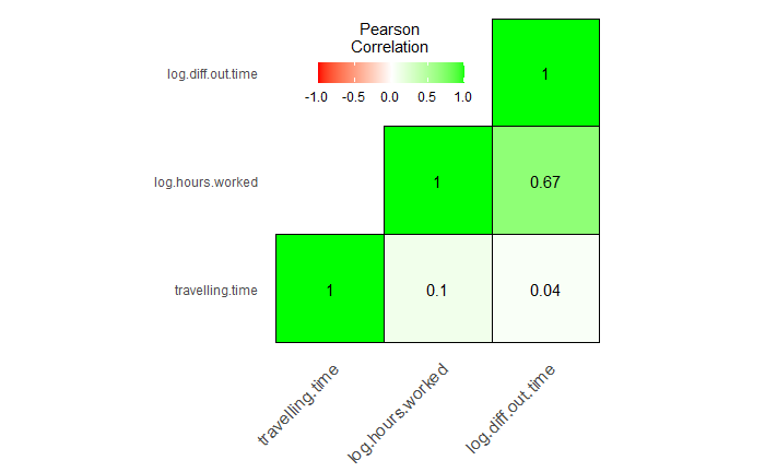
I can see that Hours worked in the previous day and the out-time of the previous day are slightly correlated(Which conceptually seems likely).
Correlation Network
Using a correlation matrix I can only check if two variables are correlated. If multiple variables are correlated, I should use Correlation Network. Even when only two variables are correlated, these plots tell me which variable among the two to keep and which to reject as a dependent variable in our model.
library("qgraph")

# Legend
Names <- c('Travelling time', 'Hours worked (previous day)', 'Previous day out time (diff)')

# Renaming variables (not necessary)
colnames(corr.variables) <- c('tr', 'hw', 'ot')

cormat <- round(cor(corr.variables), 2)
qgraph(cormat, graph = "pcor", layout = "spring", nodeNames = Names, legend.cex = 0.4)
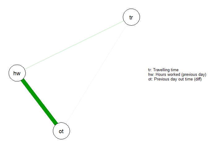
From this plot, I can see that travelling time is not correlated to any other variable, and among the other two which are correlated, I will pick out time difference as my second variable and reject hours worked.
References
- Applied Linear Statistical Models, 4th Edition
- Wikipedia (extensively)
- Correlation matrix heat map: STHDA
- Correlation network code: Sacha Epskamp
Basic statistical formulas
The formulas for some basic statistical terms used in this blog are given below.
Equation for standard deviation. $$ \sigma = \sqrt{\frac{\sum\limits_{i=1}^{n} \left(x_{i} - \bar{x}\right)^{2}} {n-1}} $$
Equation for covariance $$ cov_{x,y} = \frac{\sum\limits_{i=1}^{n}{(x_i-\overline{x}) \cdot (y_i-\overline{y})} }{n-1} $$
Created using RMarkdown