K-Means Clustering
Concept
K means clustering is the most commonly used unsupervised machine learning algorithm for partitioning a given data set into a set of k groups. It classifies objects in multiple groups (i.e., clusters), such that objects within the same cluster are as similar as possible (low intra-cluster variation), whereas objects from different clusters are as dissimilar as possible (i.e., high inter-cluster variation).
In k-means clustering, each cluster is represented by its centre (i.e. centroid).
Steps
In K-means clustering, the observations in the sample are assigned to one of the clusters by using the following steps:
1. Choose K observations from the data that are likely to be in different clusters
2. The K observations chosen in step 1 are the centroids of those clusters
3. For remaining observations, find the cluster closest to the centroid. Add the new observation (say observation j) to the cluster with the closest centroid
4. Adjust the centroid after adding a new observation to the cluster. The closest centroid is chosen based on an appropriate distance measure
5. Repeat step 3 and 4 till all observations are assigned to a cluster
The centroids keep moving when new observations are added.
Data
The data used in this blog is taken from kaggle. It is a customer segmentation problem to define market strategy. The sample Dataset summarizes the usage behaviour of about 9000 active credit card holders during the last 6 months. The file is at a customer level with 18 behavioural variables. Visit this link to know more about the data. Sample data is given below.
| CUST_ID | BALANCE | BALANCE_FREQUENCY | PURCHASES | ONEOFF_PURCHASES | INSTALLMENTS_PURCHASES | CASH_ADVANCE | PURCHASES_FREQUENCY | ONEOFF_PURCHASES_FREQUENCY | PURCHASES_INSTALLMENTS_FREQUENCY | CASH_ADVANCE_FREQUENCY | CASH_ADVANCE_TRX | PURCHASES_TRX | CREDIT_LIMIT | PAYMENTS | MINIMUM_PAYMENTS | PRC_FULL_PAYMENT | TENURE |
|---|---|---|---|---|---|---|---|---|---|---|---|---|---|---|---|---|---|
| C16568 | 3948.7769 | 1.000000 | 0.00 | 0.00 | 0.00 | 5291.215 | 0.000000 | 0.000000 | 0.000000 | 0.500000 | 17 | 0 | 4000 | 4576.5676 | 1819.1397 | 0.083333 | 12 |
| C13598 | 2104.9617 | 0.727273 | 4115.95 | 230.50 | 3885.45 | 9358.071 | 0.833333 | 0.166667 | 0.666667 | 0.916667 | 20 | 59 | 8000 | 15172.5853 | 778.2392 | 0.000000 | 12 |
| C13190 | 2089.4517 | 1.000000 | 1256.49 | 879.61 | 376.88 | 1381.853 | 0.666667 | 0.583333 | 0.500000 | 0.166667 | 2 | 32 | 2500 | 637.0447 | 1072.3948 | 0.090909 | 12 |
| C16080 | 912.9127 | 0.857143 | 0.00 | 0.00 | 0.00 | 1563.921 | 0.000000 | 0.000000 | 0.000000 | 0.285714 | 9 | 0 | 1500 | 212.0849 | 331.4871 | 0.000000 | 7 |
| C11056 | 380.3848 | 0.545455 | 1188.00 | 1188.00 | 0.00 | 0.000 | 0.083333 | 0.083333 | 0.000000 | 0.000000 | 0 | 2 | 9000 | 2461.3203 | 158.3398 | 0.000000 | 12 |
Optimal number of clusters
Identifying the optimal number of clusters is the first step in K-Means clustering. This can be done using many ways, some of which are:
1. Business decision
2. Calinski and Harabasz index
3. Silhouette statistic
4. Elbow curve
Calinski and Harabasz index
Calinhara index is an F-statistic kind of index which compares the between and within cluster variances. It is given by:
$$ CH(k) = \frac{B(k)/k-1}{W(k)/(n-k)} $$ Where k is number of clusters and B(k) and W(k) are between and within cluster variances respectively.
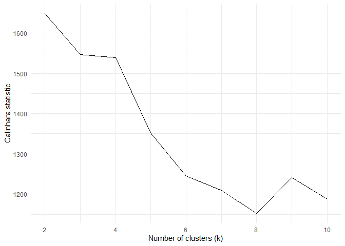
From the above plot, the ideal k value to be selected is 2.
Silhouette statistic
Silhouette statistic is the ratio of average distance within the cluster with average distance outside the cluster. If a(i) is the average distance between an observation i and other points in the cluster to which observation i belongs and b(i) is the minimum average distance between observation i and observations in other clusters. Then the Silhouette statistic is defined by
$$ S(i) = (\frac{b(i)-a(i)}{Max[a(i), b(i)]})$$ 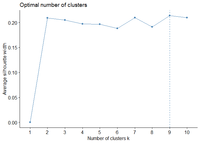
The ideal k using silhouette 2 to 6 as there is not much reduction in silhouette metric.
Elbow curve
Elbow curve is based on within-cluster variation. The location of a bend (knee) in the plot is generally considered as an indicator of the appropriate number of clusters. (see blog on hierarchical clustering for more)
fviz_nbclust(cluster_data, kmeans, method = "wss")
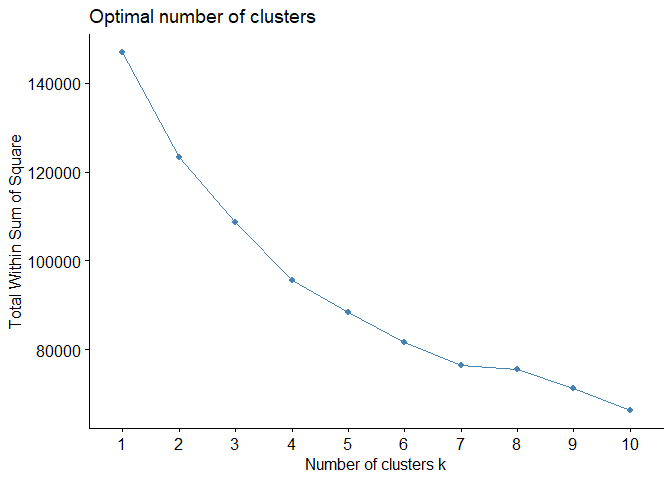
From the above three metrics, the optimum value of k is 3.
Analysing the cluster
K-means can be computed in R with the kmeans function. We will group the data into three clusters (centres = 3). The kmeans function also has a nstart option that attempts multiple initial configurations and reports on the best one. For example, adding nstart = 25 will generate 25 initial configurations. This approach is often recommended.
final_cluster <- kmeans(cluster_data, centers = 3, nstart = 25)
The final clusters can be visualized below. In the below figure, all the columns are reduced to two columns for visualization using PCA.
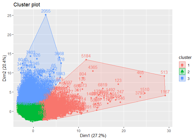
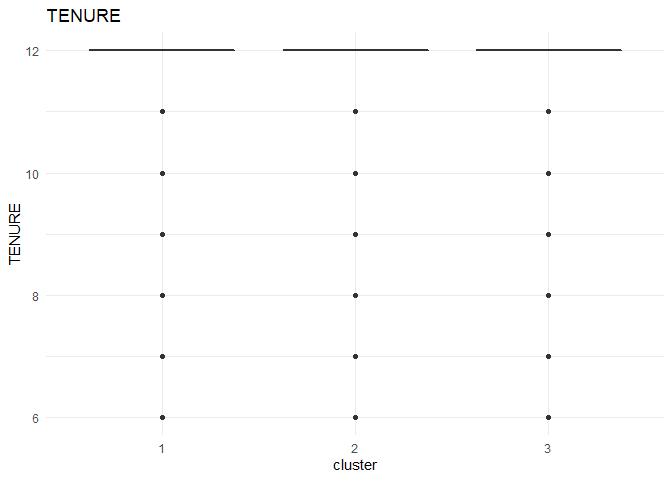
In each column, the variation between the three clusters can be analysed using the following plots. 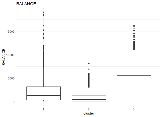
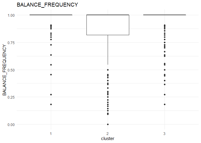
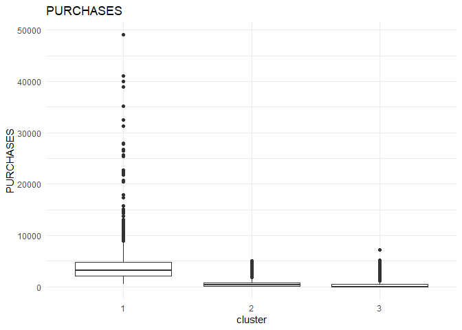
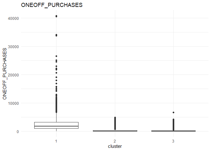
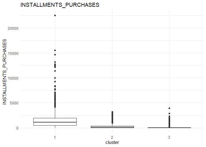
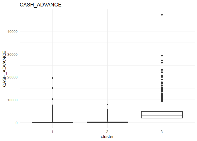
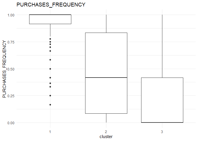
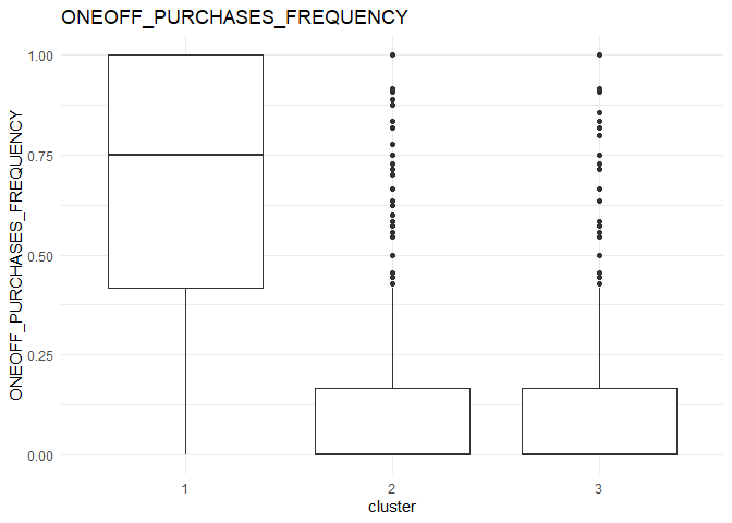
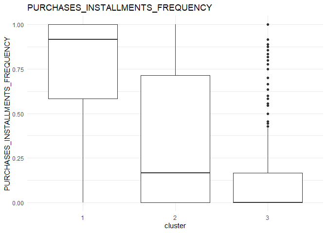
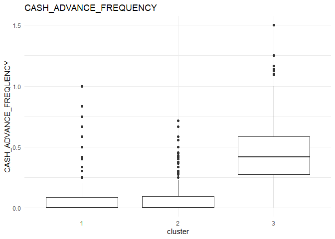
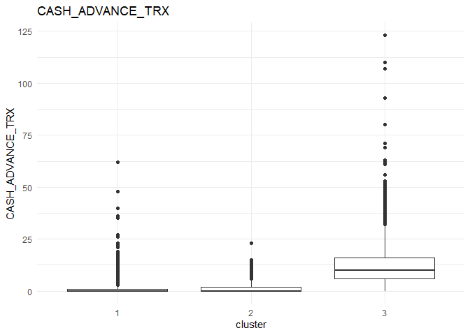
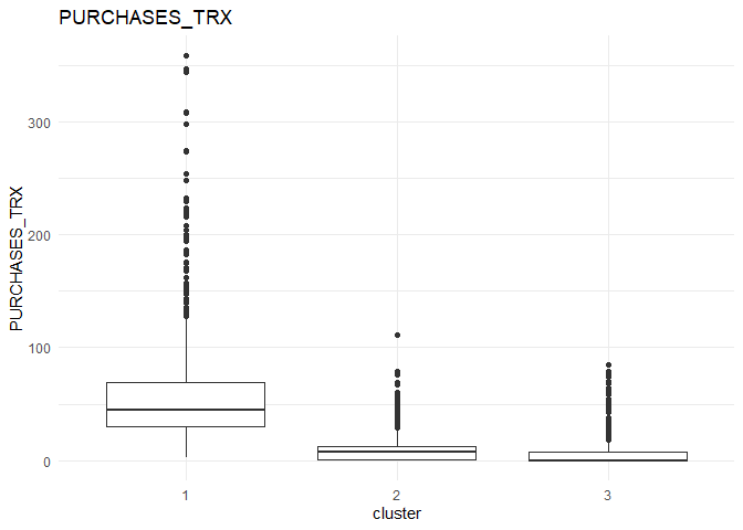
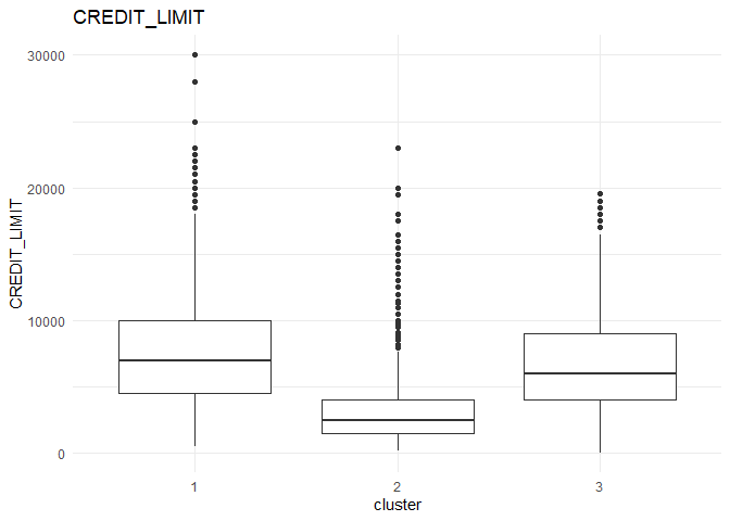
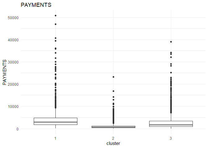
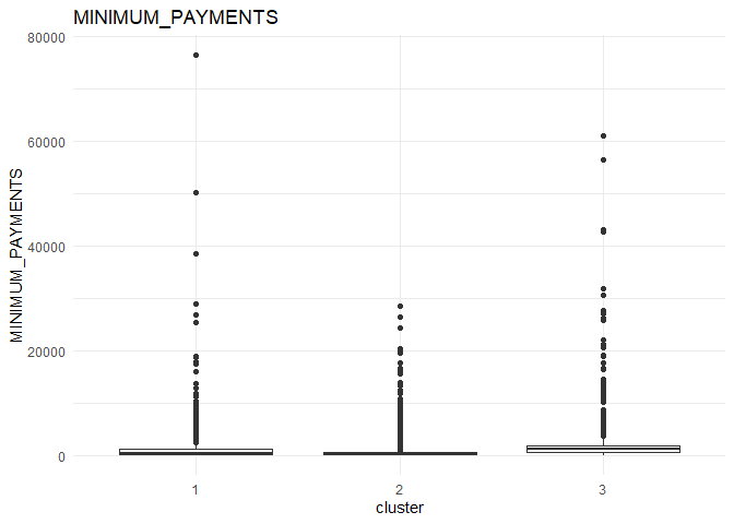
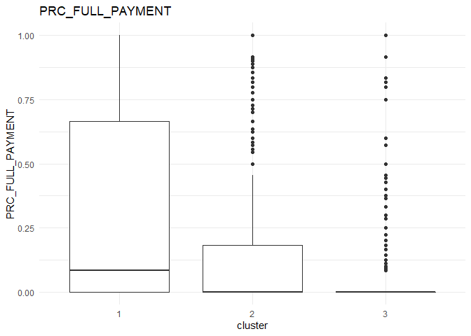
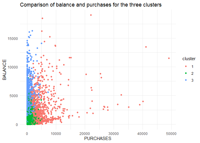
From the comparison plot, we can observe the properties of the three clusters. They are:
Cluster 1
They are customers who purchase lesser amounts using the card but have reasonably high balance in their account.
Cluster 2
They are customers who have a low balance in their account and also purchase less using the account.
Cluster 3
They are customers who purchase in higher value using their card.