Chi-Square test of independence (R)
In this post, I would like to look into Chi Square test of independence. The data set I am going to use is published in https://smartcities.data.gov.in which is a Government of India project under the National Data Sharing and Accessibility Policy.
I want to find what are the safest and deadliest ways to travel on Bangalore roads. The Injuries_and_Fatalities_Bengaluru_from_2016to2018.csv data set has the total number of injuries and fatalities in Bangalore from 2016 to 2018. I want to take injuries as a dummy for the number of incidents that took place.
As I want to test that there is significant difference in the fatalities with different types of transport, the null and alternate hypothesis will be as follows:
\(H_0\): The type of transport is independent of the fatalities
\(H_1\): The type of transport is dependent
Sample data set:
##                                                                   instance
## 1 2017 - Total Injuries - Other modes of road transport (auto, bus, lorry)
## 2                                       2018 - Total Fatalities - Bicycles
## 3                                   2017 - Total Fatalities - Two-wheelers
## 4                                     2018 - Total Fatalities - Pedestrian
## 5                                       2017 - Total Fatalities - Bicycles
##   count year             type                                        transport
## 1  1380 2017   Total Injuries Other modes of road transport (auto, bus, lorry)
## 2     9 2018 Total Fatalities                                         Bicycles
## 3    98 2017 Total Fatalities                                     Two-wheelers
## 4   276 2018 Total Fatalities                                       Pedestrian
## 5     8 2017 Total Fatalities                                         Bicycles
The contingency table for the year 2017 is
contingency_table <- data %>% filter(year == 2017) %>%
  dplyr::select(type, transport, count) %>%
  spread(type, count)
library(kableExtra)
kable(contingency_table,
      caption = 'Contingency Table') %>%
  kable_styling(full_width = F) %>%
  column_spec(1, bold = T) %>%
  collapse_rows(columns = 1:2, valign = "middle") %>%
  scroll_box()
| transport | Total Fatalities | Total Injuries |
|---|---|---|
| Bicycles | 8 | 31 |
| Other modes of road transport (auto, bus, lorry) | 252 | 1380 |
| Pedestrian | 284 | 1346 |
| Two-wheelers | 98 | 1499 |
A Mosaic plot for the same is:
library(ggmosaic)
ggplot(data = data) +
  geom_mosaic(aes(weight = count, x = product(transport), fill = type), na.rm=TRUE) +
  labs(x = 'Type of transport', y='%',  title = 'What type of transport to use') +
    theme_minimal()+theme(legend.position="bottom")
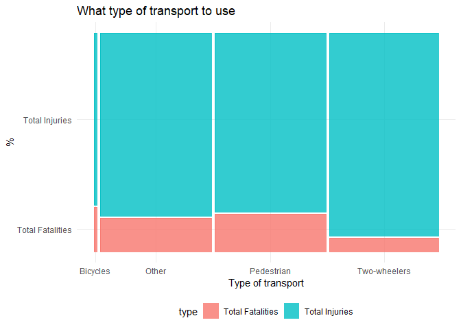
From the above plot I can observe that there is a significant difference in the percentages of fatalities in each transport. To find if this percent is significant, I will conduct a chi-square test of independence.
library(gmodels)
# Converting contingency table to flat tables
# Two vectors to hold values of columns
caseType <- c();  conditionType <- c()

# For each cell, repeat the rowname, colname combo
# as many times
for(i in 1:nrow(contingency_table)) {
  for(j in 2:ncol(contingency_table)) {
    numRepeats <- contingency_table[i, j]

    caseType <- append(caseType,
                       rep(contingency_table[i,1],
                           numRepeats))
    conditionType <- append(conditionType,
                        rep(colnames(contingency_table)[j],
                            numRepeats))
  }
}

# Construct the table from the vectors
flatTable <- data.frame(caseType, conditionType)
CrossTable(flatTable$caseType, flatTable$conditionType,
           dnn=c("Transportation Type", "Accident type"),
           expected=TRUE)
##
##
##    Cell Contents
## |-------------------------|
## |                       N |
## |              Expected N |
## | Chi-square contribution |
## |           N / Row Total |
## |           N / Col Total |
## |         N / Table Total |
## |-------------------------|
##
##
## Total Observations in Table:  4898
##
##
##                                                  | Accident type
##                              Transportation Type | Total Fatalities |   Total Injuries |        Row Total |
## -------------------------------------------------|------------------|------------------|------------------|
##                                         Bicycles |                8 |               31 |               39 |
##                                                  |            5.112 |           33.888 |                  |
##                                                  |            1.632 |            0.246 |                  |
##                                                  |            0.205 |            0.795 |            0.008 |
##                                                  |            0.012 |            0.007 |                  |
##                                                  |            0.002 |            0.006 |                  |
## -------------------------------------------------|------------------|------------------|------------------|
## Other modes of road transport (auto, bus, lorry) |              252 |             1380 |             1632 |
##                                                  |          213.913 |         1418.087 |                  |
##                                                  |            6.782 |            1.023 |                  |
##                                                  |            0.154 |            0.846 |            0.333 |
##                                                  |            0.393 |            0.324 |                  |
##                                                  |            0.051 |            0.282 |                  |
## -------------------------------------------------|------------------|------------------|------------------|
##                                       Pedestrian |              284 |             1346 |             1630 |
##                                                  |          213.650 |         1416.350 |                  |
##                                                  |           23.164 |            3.494 |                  |
##                                                  |            0.174 |            0.826 |            0.333 |
##                                                  |            0.442 |            0.316 |                  |
##                                                  |            0.058 |            0.275 |                  |
## -------------------------------------------------|------------------|------------------|------------------|
##                                     Two-wheelers |               98 |             1499 |             1597 |
##                                                  |          209.325 |         1387.675 |                  |
##                                                  |           59.206 |            8.931 |                  |
##                                                  |            0.061 |            0.939 |            0.326 |
##                                                  |            0.153 |            0.352 |                  |
##                                                  |            0.020 |            0.306 |                  |
## -------------------------------------------------|------------------|------------------|------------------|
##                                     Column Total |              642 |             4256 |             4898 |
##                                                  |            0.131 |            0.869 |                  |
## -------------------------------------------------|------------------|------------------|------------------|
##
##
## Statistics for All Table Factors
##
##
## Pearson's Chi-squared test
## ------------------------------------------------------------
## Chi^2 =  104.4776     d.f. =  3     p =  1.692478e-22
##
##
##
chi.test <- chisq.test(contingency_table[,2:3], rescale.p = TRUE)
print(chi.test)
##
##  Pearson's Chi-squared test
##
## data:  contingency_table[, 2:3]
## X-squared = 104.48, df = 3, p-value < 2.2e-16
chi.sq.plot(chi.sq = chi.test$statistic, df = chi.test$parameter, title = 'Null hypothesis to test independence')
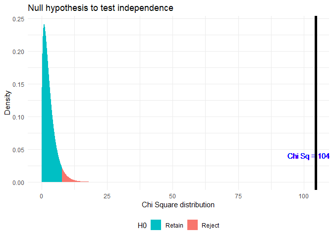
As \(p < \alpha\), where \(\alpha = 0.05\), I reject the Null hypothesis. There is a significant difference in the mortality rate with different vehicles. Travelling on two-wheeler is the safest while bicycle is the most dangerous.