Adoption of new product (R)
Introduction
Forecasting new adoptions after a product introduction is an important marketing problem. I want to use a forecasting model developed by Frank Bass that has proven to be effective in forecasting the adoption of innovative and new technologies. I am going to use Nonlinear programming to estimate the parameters of the Bass forecasting model.
Bass Forecasting model
The model has three parameters that must be estimated.
| parameter | explanation |
|---|---|
| m | the number of people estimated to eventually adopt the new product |
| q | the coefficient of imitation |
| p | the coefficient of innovation |
The coefficient of imitation (q) is a parameter that measures the likelihood of adoption due to a potential adopter being influenced by someone who has already adopted the product. It measures the “word-of-mouth” effect influencing purchases.
The coefficient of innovation (p) measures the likelihood of adoption, assuming no influence from someone who has already purchased (adopted) the product. It is the likelihood of someone adopting the product due to her or his own interest in the innovation.
If \(C_{t-1}\) is the number of people that adopted the product by time t-1, then the number of new adopters during time t is given by Bass forecasting model, and it is:
$$ F_t = (p + q[\frac{C_{t-1}}{m}])(m-C_{t-1}) $$
Data
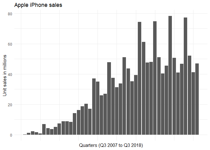
The data of iPhone sales is taken from Statista. A sample of the data is shown below.
| Quarter | Sales |
|---|---|
| Q2 '15 | 61.17 |
| Q3 '18 | 41.30 |
| Q4 '18 | 46.89 |
| Q2 '11 | 18.65 |
| Q4 '16 | 45.51 |
The sales of iPhone in different quarters can be plotted as follows:
Strictly speaking, iPhone sales for time period t are not the same as the number of adopters during time period t. But the number of repeat customers is usually small and iPhone sales is proportional to the number of customers. The Bass forecasting model seems appropriate here.
This forecasting model, can be incorporated into a nonlinear optimization problem to find the values of p, q, and m that give the best forecasts for this set of data.
Assume that N periods of data are available. Let \(S_t\) denote the actual number of adopters in period t for t = 1, . . . , N.
Then the forecast in each period and the corresponding forecast error \(E_t\) is defined by $$ F_t = (p + q[\frac{C_{t-1}}{m}])(m-C_{t-1}) = pm + (q-p)C_{t-1} - q\frac{C_{t-1}^2}{m} $$ this can be written as
\(\begin{eqnarray} F(t) &=& \beta_0 + \beta_1 \; C_{t-1} + \beta_2 \; C_{t-1}^2 \quad (BASS) \\ \beta_0 &=& pm \\ \beta_1 &=& q-p \\ \beta_2 &=& -q/m \end{eqnarray}\)
Where $$ E_t = F_t - S_t$$ Minimizing the sum of squares of errors gives me the p, q and m values. Minimizing using gradient descent, I get:
gradientDesc <- function(x1, x2, y, learn_rate, conv_threshold, n, max_iter) {
  m1 <- 0.09
  m2 <- -2*10^-5
  c <- 3.6
  yhat <- m1 * x1 + m2 * x2 + c
  MSE <- sum((y - yhat) ^ 2) / n
  converged = F
  iterations = 0
  plot(iterations, MSE, xlim = c(0, 10), ylim = c(MSE/4, MSE)) #Change this as needed
  while(converged == F) {
    ## Implement the gradient descent algorithm
    m1_new <- m1 - learn_rate * ((1 / n) * (sum((yhat - y) * x1)))
    m2_new <- m2 - learn_rate * ((1 / n) * (sum((yhat - y) * x2)))
    c_new <- c - learn_rate * ((1 / n) * (sum(yhat - y)))
    MSE <- sum((y - yhat) ^ 2) / n
    m1 <- m1_new
    m2 <- m2_new
    c <- c_new
    yhat <- m1 * x1 + m2 * x2 + c
    MSE_new <- sum((y - yhat) ^ 2) / n
    if(MSE - MSE_new <= conv_threshold) {
      converged = T
      cat("Type1: Optimal intercept:", c, "Optimal slopes:", m1, m2)
      return(c(c, m1, m2))
    }
    iterations = iterations + 1
    cat('iter', iterations, 'm1 = ', m1, 'm2 = ', m2, 'c = ', c, 'MSE = ', MSE_new, '\n')
    points(iterations, MSE_new)
    lines(x = c(iterations-1, iterations), y = c(MSE, MSE_new))
    if(iterations > max_iter) {
      abline(c, m1)
      converged = T
      return(paste("Type2: Optimal intercept:", c, "Optimal slopes:", m1, m2))
    }
  }
}
optim_param <- gradientDesc(iphone$cumulative, iphone$cumulative^2,iphone$Sales, 10^-12, 0.001, 46, 2500)
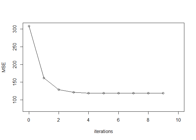
## iter 1 m1 =  0.08999999 m2 =  -2.991878e-05 c =  3.6 MSE =  162.2441
## iter 2 m1 =  0.08999999 m2 =  -3.46669e-05 c =  3.6 MSE =  128.9074
## iter 3 m1 =  0.08999999 m2 =  -3.693982e-05 c =  3.6 MSE =  121.2682
## iter 4 m1 =  0.08999999 m2 =  -3.802787e-05 c =  3.6 MSE =  119.5177
## iter 5 m1 =  0.08999999 m2 =  -3.854871e-05 c =  3.6 MSE =  119.1165
## iter 6 m1 =  0.08999999 m2 =  -3.879804e-05 c =  3.6 MSE =  119.0246
## iter 7 m1 =  0.08999999 m2 =  -3.89174e-05 c =  3.6 MSE =  119.0035
## iter 8 m1 =  0.08999999 m2 =  -3.897453e-05 c =  3.6 MSE =  118.9987
## iter 9 m1 =  0.08999999 m2 =  -3.900189e-05 c =  3.6 MSE =  118.9976
## Type1: Optimal intercept: 3.6 Optimal slopes: 0.08999999 -3.901498e-05
From the above slope values, I can get the p, q and m values:
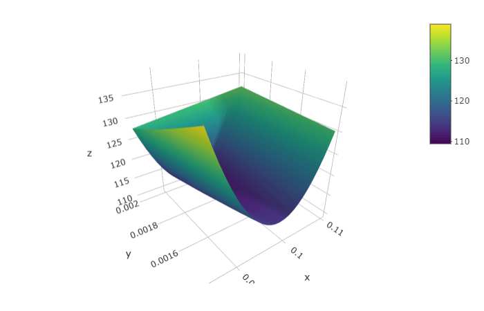
## The optimum for m, p and q are 2346.136 0.001534438 0.09153443
The objective function is plotted as below.
Sales Peak
It is easy to calculate the time at which adoptions will peak out. The peak sales is given by \(t^* = \frac{-1}{p+q}\; \ln(p/q)\)
## [1] 47.52522
Sales Forecast
We cal also try to forecast the sales in the future 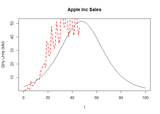
Wrap up
There are two ways in which the Bass forecasting model can be used:
1. Assume that sales of the new product will behave in a way that is similar to a previous product for which p and q have been calculated and to subjectively estimate m, the potent forecast for period 7 is made. This method is often called a rolling-horizon approach.
2. Wait until several periods of data for the new product are available. For example, if five periods of data are available, the sales data for these five periods could be used to forecast demand for period 6. Then, after six periods of sales are observed,
References
- Data Science: Theories, Models, Algorithms, and Analytics - Sanjiv Ranjan Das online
- A New Product Growth for Model Consumer Durables - Bass Management Science, January 1969
- An Introduction to Management Science : Quantitative Approach to Decision Making - Anderson and Sweeney Cengage
- Linear regression using gradient descent online
- Prof Gila E. Fruchter notes online
- Apple iPhone sales - statistica online
- Gradient descent - towardsdatascience online
- Implementation in R - r-bloggers online