VAR Models (R)
Forecasting demand in brick and motor stores
One of the main problems that brick and mortar retailers face is forecasting demand. In retail stores, people usually buy multiple products with a large range across a variety of products. Sales of different products are correlated, for example, if a family is buying at the start of the month, they would buy all household groceries which span various products and ranges. Take another example of young fathers buying wine and diapers together at Walmart[1], or people who buy milk also buy bread. These cross-correlations in the demand make predicting demand difficult. For example, the demand for socks is also correlated with shoes, and therefore for predicting the demand for shoes, we should consider the demand for both shoes and socks from the previous periods. This makes demand forecasting more complex in retail stores as in a typical regression, these cross-correlation effects are not taken into consideration. Dual causality and complex feedback loops between the sales in departments are not considered in typical regression and demand forecasts. In this blog, we use Walmart's data to predict sales (after marketing) at various departments. The results for one particular store are taken and analysed in detail to explain in detail.
Data
The data used is taken from "Walmart Recruiting - Store Sales Forecasting data competition" on Kaggle[2]. This contains sales and marketing data for 99 departments and 45 stores from 2010 to 2012. At every store, external factors like CPI, unemployment, temperature, fuel price and holidays are given. Additionally, four different markdowns are given at the store level from the date 11-11-2011.
##   Store       Date Temperature Fuel_Price MarkDown1 MarkDown2 MarkDown3
## 1    18 2011-05-20       57.55      4.101        NA        NA        NA
## 2    40 2011-01-14       18.55      3.215        NA        NA        NA
## 3     9 2010-11-26       60.18      2.735        NA        NA        NA
## 4    35 2010-02-26       36.00      2.754        NA        NA        NA
## 5     1 2013-02-08       56.67      3.417  32355.16     729.8    280.89
##   MarkDown4 MarkDown5      CPI Unemployment IsHoliday
## 1        NA        NA 134.6804        8.975     FALSE
## 2        NA        NA 132.9511        5.114     FALSE
## 3        NA        NA 215.2909        6.560      TRUE
## 4        NA        NA 135.5195        9.262     FALSE
## 5  20426.61   4671.78 224.2350        6.525      TRUE
Department-store level sales data is also provided for every week.
##   Store Dept       Date Weekly_Sales IsHoliday
## 1    29   74 2011-02-11      8160.66      TRUE
## 2    45   71 2010-10-01      3399.40     FALSE
## 3    20   91 2011-02-18     86224.01     FALSE
## 4    20    5 2011-11-04     48799.61     FALSE
## 5    32   41 2012-03-16      1396.00     FALSE
Assumptions
In this analysis, the assumptions are as follows:
1. Considering only fast-moving departments: Fast-moving departments are defined as departments that have at least one item sold every day in every store. Predicting demand for slow-moving items, especially when the items are not sold at all for a few days is complex and requires a different analysis. We should check if the sales follow a Poisson distribution and model the difference of time between sales using an exponential distribution (which we are not doing in this analysis).
2. Ignoring the smaller cross-correlations between sales of departments.
3. The VAR model has an additive form. This means that the effect of cross-correlations is additive.
4. Markdowns are considered endogenous variables as the sales increase due to markdowns are present only in that period and do not spill over when the markdowns are not present.
Methodology
The sales across different departments are visualized and classified into fast-moving and slow-moving departments. Fast-moving departments are departments that have at least one item sold every day in each store. Based on correlations among the fast-moving departments, four clusters are formed. After testing for stationarity, to model sales, a VAR(1) model with sales of all the departments (in the cluster) as exogenous variables and markdowns, temperature and other demographic variables as endogenous variables is built. This model at a store level is used to predict sales of the departments in the clusters. VAR model is used to model the complex loops caused due to the correlation in sales between the departments (within a cluster). This is extended to all stores across all department clusters to predict the sales for the future.
Analysis
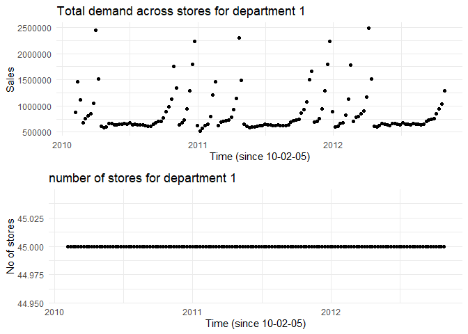
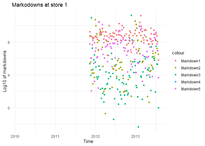
Scatter plots (appendix) show the total sales of the department (all stores combined) across time. The count of stores is added to identify fast-moving departments. There are a total of five types of markdowns that were active across the stores. While the markdowns are not given at the department level, we assume that markdowns affect sales across departments due to cross-correlations. The magnitude of these markdowns is plotted for each store (appendix). This shows that in almost all stores, Markdown 1 is the highest while Markdown 3 is the lowest.
From the plots above, we are restricting our analysis to the following departments 1, 2, 3, 4, 7, 10, 13, 14, 16, 21, 30, 38, 40, 46, 67, 79, 81, 82, 90, 91, 92, 95 as they are fast-moving. We also observe that there is no visible pattern among the markdowns. This indicates that predicting the markdowns for the past (where we have missing data) would be challenging.
The correlations between the total sales of the department's can be visualized in the below correlation plot.
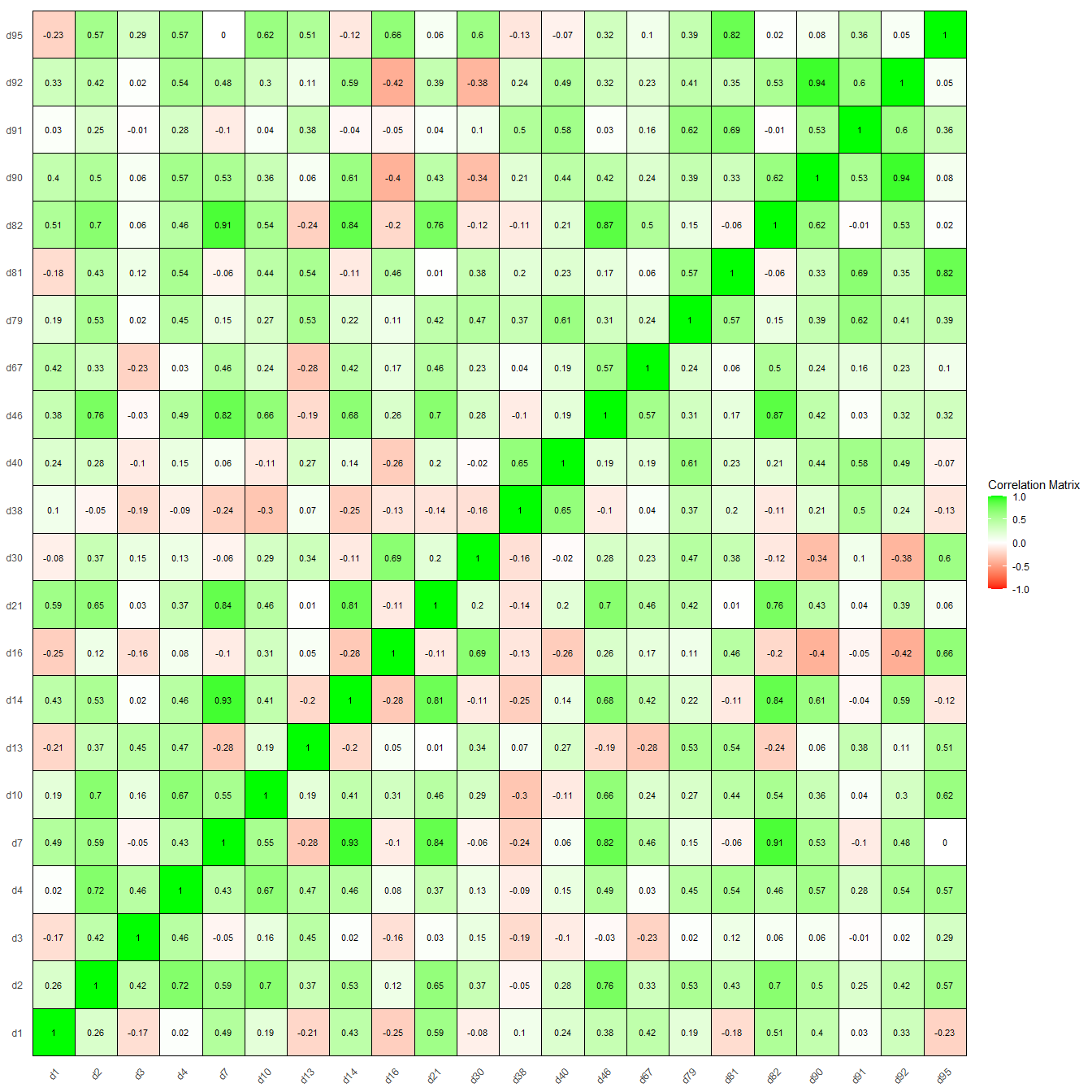
These correlations can be used to create clusters of departments that are closely related using hierarchical clustering. Four clusters are created with minimum 3 and maximum 7 departments.
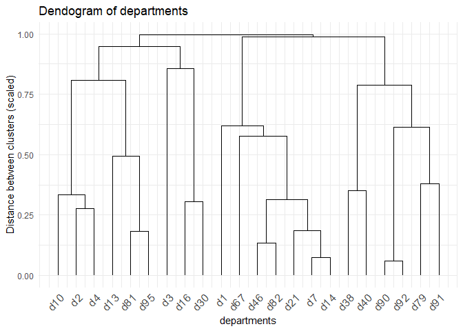 The four clusters are
# Four clusters
c1 <- c(10, 2, 4, 13, 81, 95)
c2 <- c(3, 16, 30)
c3 <- c(1, 67, 46, 82, 21, 7, 14)
c4 <- c(38, 40, 90, 92, 79, 91)
The assumption is that the sales of the departments within the cluster have cross-correlations and are dependent on each other, with no influence from departments outside the cluster.
In the next step, we test the stationarity of the sales in each department. The analysis for cluster 1 is demonstrated, and a similar analysis should be carried out for the remaining clusters.
Cluster 1
With the assumption that the sales in the departments that are within cluster-1 are correlated and the departments outside the cluster do not affect the sales of the departments within the cluster, we can try to build a VAR model with department sales as exogenous variables. The first step to build a VAR model is to perform a unit root test to identify if the sales are stationary. The most common tests to test stationarity are KPSS and ADF tests. In this analysis, KPSS tests are performed, and for each department, the following steps are carried out.
1. If the data is stationary, the data is not modified. This data is represented by 'd'+department number
2. If the data is not found to be stationary, differencing is done to bring the data to stationarity and the differenced data is represented as 'Dd' + department number
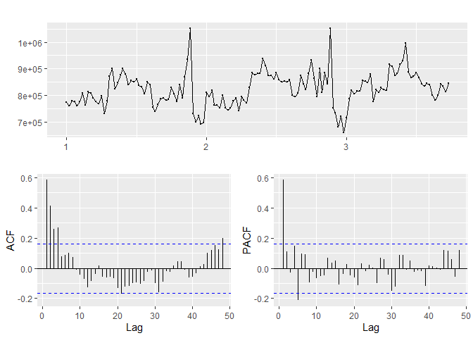
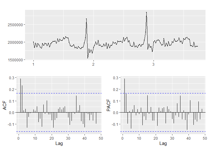
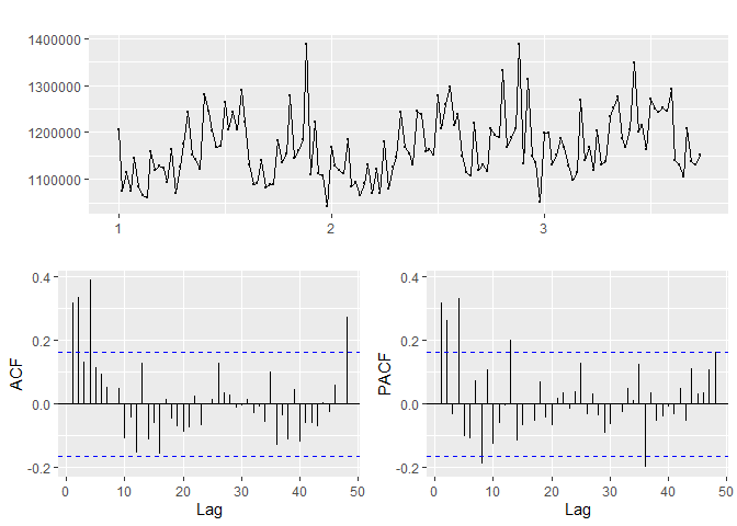
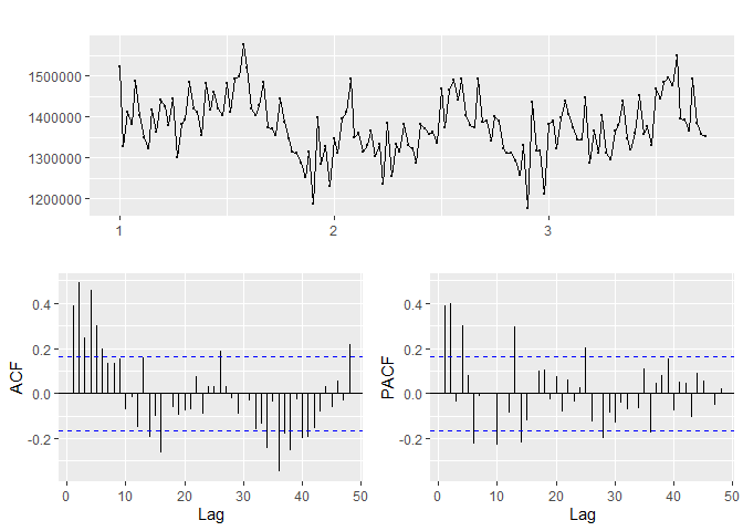
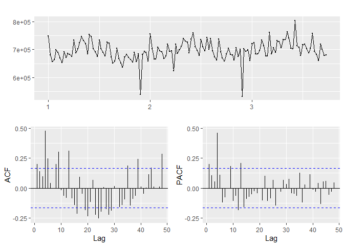
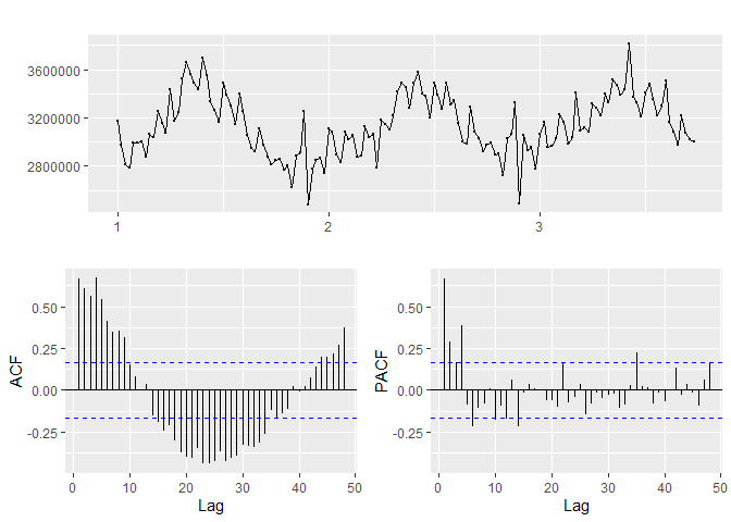
The KPSS test result, time series plot, ACF and PACF plots are shown for each department in cluster 1. Note, the total sales of the department (Combining all stores) is taken for the analysis. The final data (after converting to stationary) for each department is also shown.
## [1] "Department 10"
##
##  KPSS Test for Level Stationarity
##
## data:  time.series.ts
## KPSS Level = 0.37175, Truncation lag parameter = 4, p-value = 0.08933
##
## [1] "The ideal differencing parameter is 1"
## [1] "_____"
## [1] "Department 2"
##
##  KPSS Test for Level Stationarity
##
## data:  time.series.ts
## KPSS Level = 0.19425, Truncation lag parameter = 4, p-value = 0.1
##
## [1] "The ideal differencing parameter is 0"
## [1] "_____"
## [1] "Department 4"
##
##  KPSS Test for Level Stationarity
##
## data:  time.series.ts
## KPSS Level = 0.51039, Truncation lag parameter = 4, p-value = 0.03933
##
## [1] "The ideal differencing parameter is 1"
## [1] "_____"
## [1] "Department 13"
##
##  KPSS Test for Level Stationarity
##
## data:  time.series.ts
## KPSS Level = 0.25715, Truncation lag parameter = 4, p-value = 0.1
##
## [1] "The ideal differencing parameter is 1"
## [1] "_____"
## [1] "Department 81"
##
##  KPSS Test for Level Stationarity
##
## data:  time.series.ts
## KPSS Level = 0.33434, Truncation lag parameter = 4, p-value = 0.1
##
## [1] "The ideal differencing parameter is 1"
## [1] "_____"
## [1] "Department 95"
##
##  KPSS Test for Level Stationarity
##
## data:  time.series.ts
## KPSS Level = 0.19382, Truncation lag parameter = 4, p-value = 0.1
##
## [1] "The ideal differencing parameter is 0"
## [1] "_____"
## # A tibble: 6 x 7
##   Date          Dd10       d2      Dd4     Dd13    Dd81      d95
##   <chr>        <dbl>    <dbl>    <dbl>    <dbl>   <dbl>    <dbl>
## 1 2010-02-05     NA  1997832.      NA       NA      NA  3170530.
## 2 2010-02-12 -11344. 1839218. -130720. -195422. -67271. 2976149.
## 3 2010-02-19  17950. 1961686.   38700.   85263. -22911. 2814038.
## 4 2010-02-26  -3917. 1859532.  -37947.  -30634    7311. 2789412.
## 5 2010-03-05 -13688. 1957871.   69672.  106626.  33480. 2994339.
## 6 2010-03-12  15532. 1908498.  -61575.  -83957.  -8533. 2992259.
Based on the p-values in the KPSS test, departments 10, 4 are not-stationary while departments 2, 13, 81 and 95 are stationary.
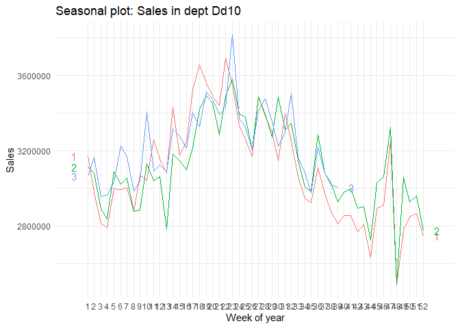
Testing for seasonality
Despite making the data stationary, we can still see seasonality in some departments. As we do not have data (at least three years of data to find patterns), we are ignoring seasonality. We assume that the increase in sales in particular seasons is due to holidays. We have holidays as a proxy for some seasonal patterns. In the below plots, these seasonalities are shown.
Analysis in one store
While in the previous analysis, we have looked at the total sales of the department and identified the trends of each department, we want to predict the sales for each store. Assuming that the behaviour of the departments is similar across stores we can build VAR models for each store and department cluster. This assumption means that the correlations and clusters between departments remain the same across all stores and the departments will have the same stationary patterns across stores. In the current analysis, we demonstrate the analysis for one store (and one cluster). Similar analysis can be scaled up for multiple stores and department clusters.
Null value treatment: In the data provided, there are three types of Null values.
1. For temperature, Fuel price, unemployment and CPI index, the null values are replaced with mean values in the store. This is because there is a small deviation of these numbers within a store. Assuming that the mean will be close to the actual number of these variables would be reasonable. These values do not follow a pattern and are random.
2. For markdowns after 11-11-11, null values are replaced with Zero. For markdown data after 11-11-11, any null value is assumed to be present due to no markdowns.
3. For markdowns before 11-11-11, null values are imputed with zero. This is the timeframe where we do not have reliable data. As discussed in the EDA, it is difficult to extrapolate markdowns data to the past due to a lack of sufficient length of data.
VAR Model
The last step in the model building process is to build a VAR model on the data. In the VAR(1) model, the departments (after bringing to stationarity) are exogenous variables and customer demographics and markdowns are endogenous variables. The VAR(1) model will have the following equation.
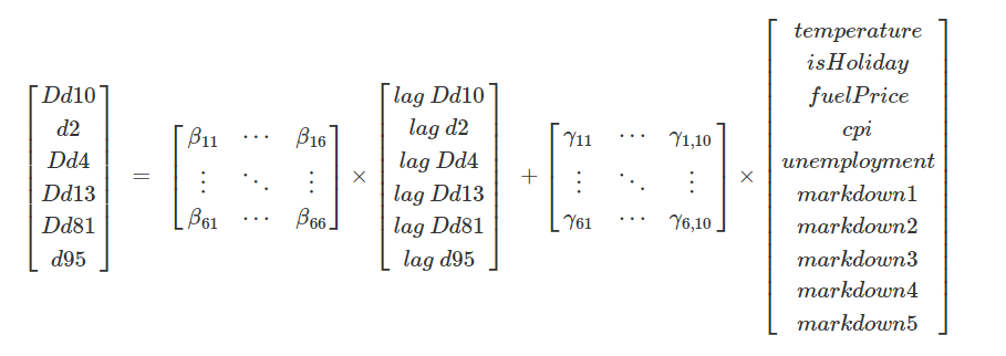
In this formula, \(\beta_{xy}\) values indicate the effect due to cross correlation between variable x and y (if \(x \neq y\)). if \(x=y\) in \(\beta_{xy}\), they represent the effect of lag of the variable in the sales.
##
## ============================================================================================================
##                                                             Dependent variable:
##                                -----------------------------------------------------------------------------
##                                    Dd10          d2          Dd4          Dd13         Dd81         d95
##                                    (1)          (2)          (3)          (4)          (5)          (6)
## ------------------------------------------------------------------------------------------------------------
## Dd10.l1                         -0.286***      0.114        0.010        0.080        0.025        0.324*
##                                  (0.092)      (0.090)      (0.083)      (0.064)      (0.049)      (0.193)
##
## d2.l1                             -0.184      0.531***      -0.099       -0.055       0.075       0.724***
##                                  (0.117)      (0.115)      (0.106)      (0.082)      (0.063)      (0.248)
##
## Dd4.l1                            0.009        0.001        -0.146       0.082      -0.263***    -1.169***
##                                  (0.132)      (0.130)      (0.119)      (0.092)      (0.071)      (0.278)
##
## Dd13.l1                           -0.037       -0.197       -0.152     -0.438***     0.204***      0.351
##                                  (0.126)      (0.124)      (0.114)      (0.088)      (0.068)      (0.266)
##
## Dd81.l1                           0.187        -0.179       -0.083      -0.286**      0.159       1.668***
##                                  (0.205)      (0.201)      (0.184)      (0.142)      (0.110)      (0.431)
##
## d95.l1                          -0.173***    -0.145***    -0.185***    -0.165***    -0.192***      -0.166
##                                  (0.050)      (0.049)      (0.045)      (0.035)      (0.027)      (0.105)
##
## const                           1,259.417   -58,338.040  -63,432.750   12,448.240  -32,166.350  -83,971.470
##                                (45,763.050) (44,936.070) (41,248.780) (31,835.530) (24,562.400) (96,508.170)
##
## temperature1                    83.640***     51.626*     82.132***    85.331***    75.216***    510.080***
##                                  (31.272)     (30.707)     (28.187)     (21.755)     (16.785)     (65.949)
##
## isHoliday1                     3,057.221**  -2,391.432*   1,732.907     497.243      -936.931    -2,613.765
##                                (1,290.046)  (1,266.733)  (1,162.790)   (897.433)    (692.406)   (2,720.534)
##
## fuelPrice1                       196.925     -1,152.437    -796.645     393.762      -166.682    1,297.270
##                                (1,089.316)  (1,069.631)   (981.861)    (757.793)    (584.668)   (2,297.221)
##
## markdown1                        0.213**       0.132        0.179*       0.116        0.082        0.238
##                                  (0.103)      (0.101)      (0.093)      (0.072)      (0.055)      (0.217)
##
## markdown2                         -0.032     -0.226***     -0.143**      0.031       -0.084**     -0.383**
##                                  (0.073)      (0.072)      (0.066)      (0.051)      (0.039)      (0.154)
##
## markdown3                         -0.036       0.006        0.098*       0.021        0.019        -0.015
##                                  (0.063)      (0.062)      (0.056)      (0.044)      (0.034)      (0.132)
##
## markdown4                         -0.026       0.119        -0.047       0.051        -0.033       -0.091
##                                  (0.115)      (0.113)      (0.104)      (0.080)      (0.062)      (0.242)
##
## markdown5                         0.001        -0.072     -0.323***      -0.105       -0.113       -0.128
##                                  (0.130)      (0.127)      (0.117)      (0.090)      (0.070)      (0.273)
##
## cpi1                              51.748      354.970*    352.551**      15.173      199.652*     675.145*
##                                 (192.152)    (188.680)    (173.197)    (133.673)    (103.134)    (405.223)
##
## unemployment1                   1,289.625   2,745.903**   1,477.331     -87.638      567.653      873.228
##                                (1,323.139)  (1,299.229)  (1,192.619)   (920.455)    (710.168)   (2,790.324)
##
## ------------------------------------------------------------------------------------------------------------
## Observations                       141          141          141          141          141          141
## R2                                0.339        0.324        0.472        0.577        0.482        0.646
## Adjusted R2                       0.254        0.237        0.404        0.522        0.416        0.600
## Residual Std. Error (df = 124)  3,061.286    3,005.966    2,759.307    2,129.614    1,643.083    6,455.843
## F Statistic (df = 16; 124)       3.978***     3.723***     6.940***    10.563***     7.223***    14.119***
## ============================================================================================================
## Note:                                                                            *p<0.1; **p<0.05; ***p<0.01
Conclusions
Statistical observations: The F-statistics for the model of all the dependent variables are significant at a 5% confidence interval. The R^2 metrics are between 32-65% indicating the percentage of demand variation that is explained by the model. Temperature is significant in all the departments. holidays are significant only in departments 10 and 2 while fuel price is not significant in any department. CPI is not-significant in departments 10 and 13 while unemployment is significant in department 2 only. Among markdowns, the first markdown is significant only for departments 10 and 4, the second for 2, 13, 81 and 95, the third and fourth markdowns are not significant, and the fifth one is significant in the department 4.
From the significant variables, we can observe the following:
1. Temperature is a good proxy for seasonality. To improve the prediction, classifying temperature into different ranges might help.
2. Departments 10 and 2 have a lot of products that are commonly given as gifts during the holiday seasons. During the holiday season, these departments should be given more focus.
3. The demand for items in departments 10 and 13 is resilient to small changes in inflation and CPI. This could mean that these items might be inelastic.
4. The products in department 2 have higher sales while a customer is unemployed.
5. Not all markdowns affect the sales of different departments. For example, Markdown type 1 is useful to improve the sales of departments 10 and 4 only. More analysis on the nature of markdowns is required to understand the reasons for this trend. Markdowns can be planned more efficiently if these relationships can be analysed further. We can ask questions like "do markdowns (of type 1) on shoes improve the sales of socks", and "Can I create markdowns or discounts with products across departments like a discount if shoes and socks are brought together. The effect of some markdowns is negative in some departments (in presence of other markdowns). This has to also be investigated. Sometimes, providing markdowns for some items can improve the sales in that department/product but cannibalises sales in other departments/products.
6. Department 13 is not influenced by any markdowns, indicating this could be a department of inelastic products. Walmart can relook at the pricing strategy for these items.
The demand equation for the demand of department 95 at store 1 is as follows (only significant variables).
$$ demand_{95, t} = 0.324\times \Delta sales_{10, t-1} + 0.724\times sales_{2, t-1} -1.169\times \Delta sales_{4, t-1} +1.668\times \Delta sales_{81, t-1} + 0\times sales_{95, t-1} + 510\times temperature_t - 0.383\times markdown2_{t} + 675.14\times cpi_{t} -83971$$ From this equation, we can see that sales of products in department 2 in the previous period have a positive impact (if one hundred additional items were sold in the previous period in department 2, 72 additional units will be sold in department 95). Similarly, departments 13 and 81 also have a positive impact on sales. Department 4 has a negative impact on sales (for one additional unit increase in sales in department 4, the sales in the current period decreased by 1.16 units). The previous period demand has no significance (in presence of other variables).
Predictions
Finally, using the VAR(1) model, we can predict the demand in each department for different values of markdowns and other exogenous variables. For example, with the same markdowns and demographic values the demand prediction for the next 10 time periods is provided. Additionally, their confidence intervals are also provided.
##  [1] 1907.21184 1392.08756 1121.89931 -926.18603  -50.90932 -937.08478
##  [7] -527.70790  244.23242 -403.57184 -469.50484
Ending
The above analysis demonstrates how to forecast demand when correlations between different departments/products exist. We have also looked into the effect of different types of markdowns on different departments. Analysing further into the details of the markdowns can help us design markdowns more efficiently. We have also seen that temperature can be a proxy for seasonality in the data. Finally, we have shown how the demand for different products/departments affects demand due to cross-correlations and how to model them.
References
Appendix