Seasonal time series (R)
Data and context
This blog is inspired by the work done at www.andreasgeorgopoulos.com for predicting the demand for lettuce in a particular store (46673) fast food chain of restaurants. The data and EDA for the same can be found in the above link. You can find the same in my git repository.
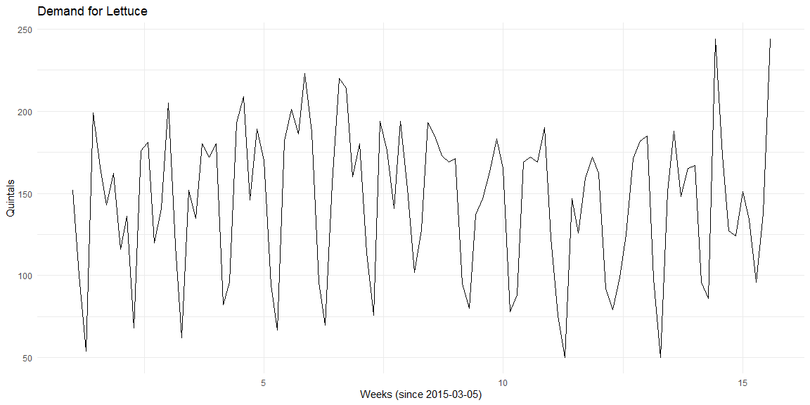
The historical demand for Lettuce for the first ten days is shown below.
| date | IngredientId | quantity_lettuce |
|---|---|---|
| 15-03-05 | 27 | 152 |
| 15-03-06 | 27 | 100 |
| 15-03-07 | 27 | 54 |
| 15-03-08 | 27 | 199 |
| 15-03-09 | 27 | 166 |
| 15-03-10 | 27 | 143 |
| 15-03-11 | 27 | 162 |
| 15-03-12 | 27 | 116 |
| 15-03-13 | 27 | 136 |
| 15-03-14 | 27 | 68 |
Demand forecasting with Seasonality
The Lettuce in store 46673 shows a clear seasonal pattern. The quantity of Lettuce used seems to depend on the day of the week. From this plot, there seems to be no discernible trend in the quantity of Lettuce used.
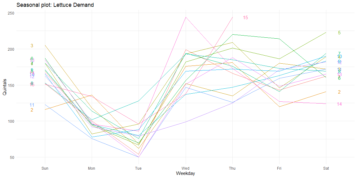
Visualising seasonality
We can visualise this seasonality using seasonal plots. From these plots, we can see that the demand for Lettuce is the least on Tuesday while highest on Wednesdays. Thus, a clear weekly seasonality in the data can be observed in the data.
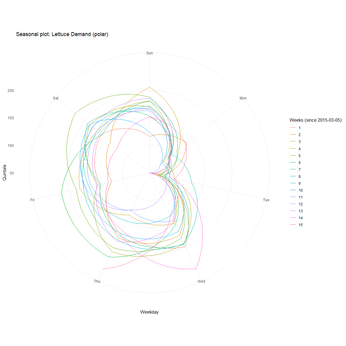
The same is more evident in polar coordinates.
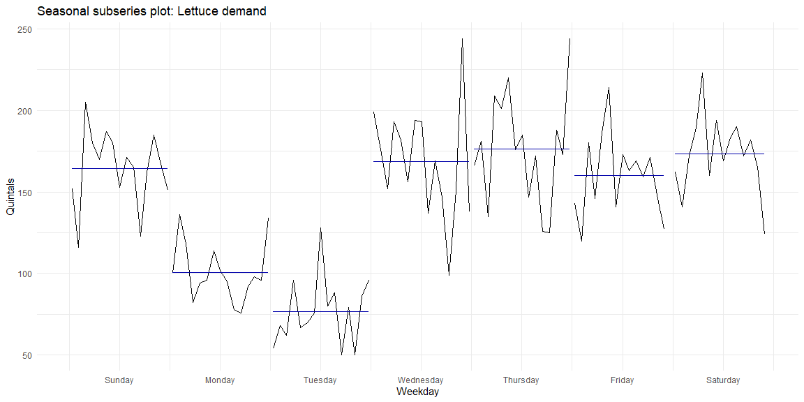
We can see the similarity in demand within weekdays by looking at the seasonal subseries plots where data for each weekday is collected together. The mean and the variance across weeks for each of the weekdays can be seen.
SARIMA
As the data is seasonal, we will need to use SARIMA (Seasonal ARIMA). By looking at these plots, I suspect that the series is stationary. This can be validated using Dickey-Fuller and KPSS tests.
Dickey−Fuller Test
Dickey−Fuller test is a hypothesis test in which the null hypothesis and alternative hypothesis are given by
\(H_0\): \(\gamma\) = 0 (the time series is non-stationary)
\(H_1\): \(\gamma\) < 0 (the time series is stationary)
Where $$ \Delta y_t = \alpha + \beta t + \gamma y_{t-1} + \delta_1 \Delta y_{t-1} + \delta_2 \Delta y_{t-2} + \dots $$
##
##  Augmented Dickey-Fuller Test
##
## data:  time.series
## Dickey-Fuller = -8.4973, Lag order = 4, p-value = 0.01
## alternative hypothesis: stationary
KPSS Test
The null hypothesis for the KPSS test is that the data is stationary.
##
##  KPSS Test for Trend Stationarity
##
## data:  time.series
## KPSS Trend = 0.10896, Truncation lag parameter = 4, p-value = 0.1
ACF and PACF plots
The ACF and PACF plots of this time series are:
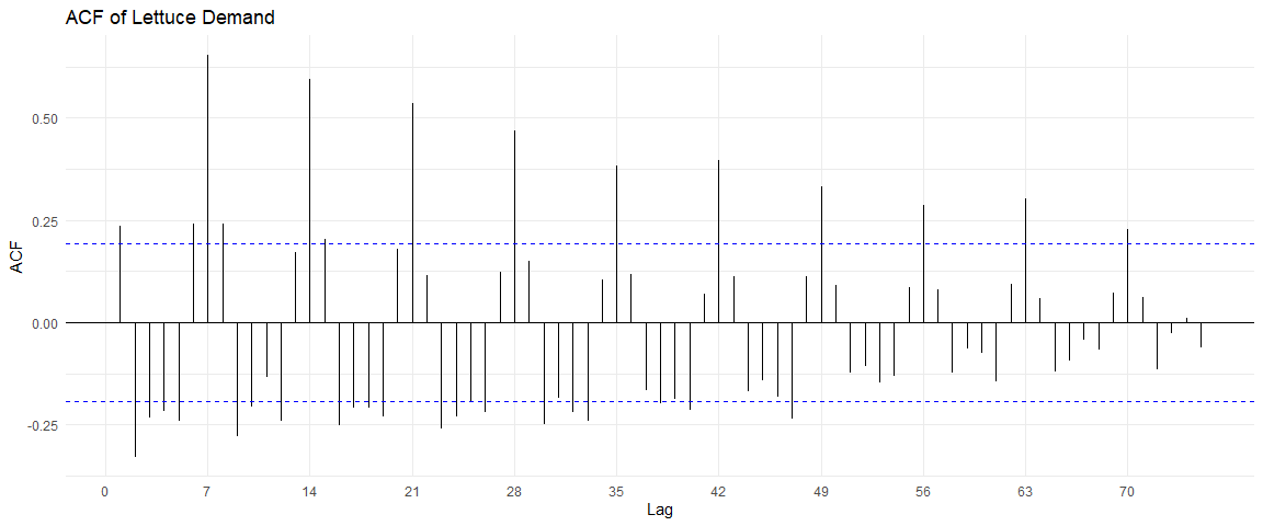
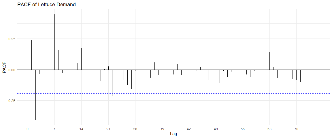
From the ACF plot, I can see a correlation within multiples of 7, indicating a weekly seasonality. However, the PACF shows no such trend after the first iteration.
Stationarity in the seasonal component
To test if the seasonal component is also stationary, we can look at the time series after differencing with period 7 (which will remove the seasonal non-stationarity if it exists).
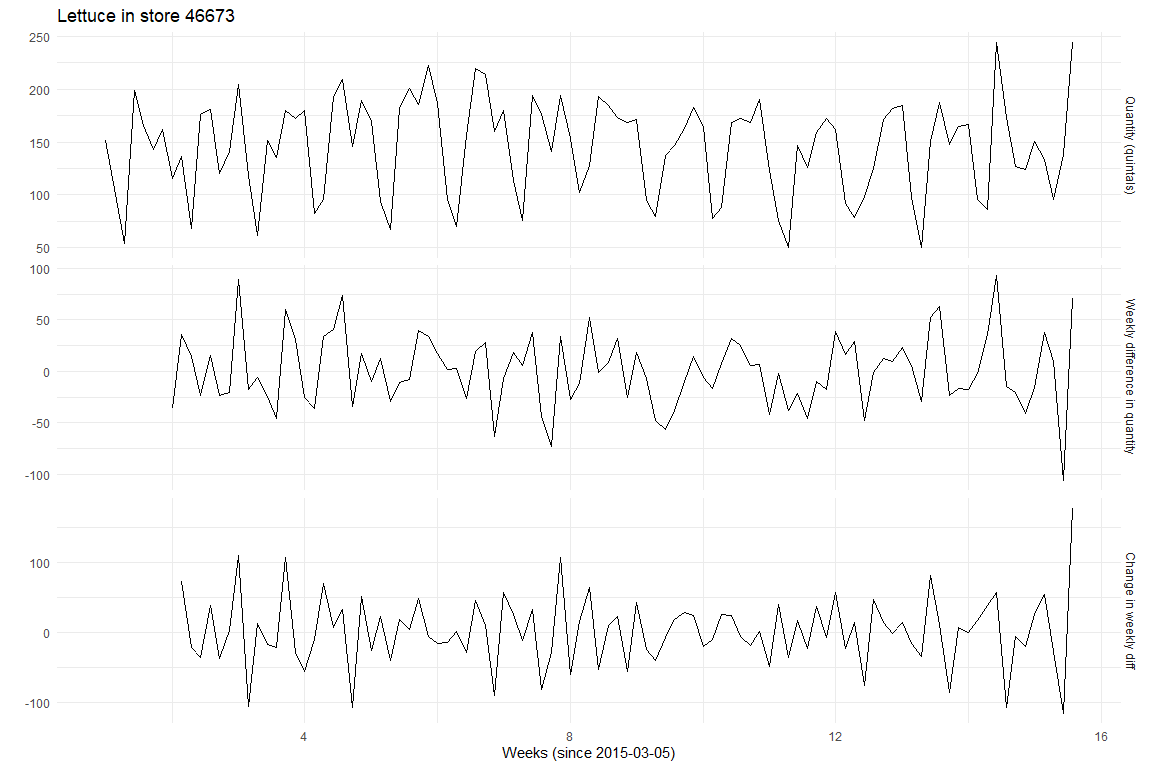
After differencing once with period 7, we can determine if the data is still stationary using the KPSS test. We can also use the nsdiff function in R to find the differencing factor to make the data stationary.
library(urca)
diff(time.series,7) %>% ur.kpss %>% summary()
##
## #######################
## # KPSS Unit Root Test #
## #######################
##
## Test is of type: mu with 3 lags.
##
## Value of test-statistic is: 0.0759
##
## Critical value for a significance level of:
##                 10pct  5pct 2.5pct  1pct
## critical values 0.347 0.463  0.574 0.739
# Number of differencing necessary on the data to bring to stationarity
time.series %>% nsdiffs()
## [1] 1
# After differencing with period 7, we are checking for stationarity
time.series %>% diff(lag=7) %>% nsdiffs()
## [1] 0
Auto Sarima
We can minimize AIC and BIC to find the optimal (p, d, q) coefficients, as well as the seasonal (p, d, q) components.
To reduce over-fitting, we can reduce the data into training and test datasets. We will use the train dataset to train, and compare the accuracy on the test dataset. As we have around 15 weeks of data (15th week is not full), we can use the first 13 weeks for training and the remaining 14th and 15th week for testing.
##
##  ARIMA(2,0,2)(1,1,1)[7] with drift         : 810.332
##  ARIMA(0,0,0)(0,1,0)[7] with drift         : 835.2064
##  ARIMA(1,0,0)(1,1,0)[7] with drift         : 814.9145
##  ARIMA(0,0,1)(0,1,1)[7] with drift         : 803.1689
##  ARIMA(0,0,0)(0,1,0)[7]                    : 833.1092
##  ARIMA(0,0,1)(0,1,0)[7] with drift         : 837.2882
##  ARIMA(0,0,1)(1,1,1)[7] with drift         : 805.3521
##  ARIMA(0,0,1)(0,1,2)[7] with drift         : 805.3646
##  ARIMA(0,0,1)(1,1,0)[7] with drift         : 814.7505
##  ARIMA(0,0,1)(1,1,2)[7] with drift         : Inf
##  ARIMA(0,0,0)(0,1,1)[7] with drift         : 803.6079
##  ARIMA(1,0,1)(0,1,1)[7] with drift         : 805.3438
##  ARIMA(0,0,2)(0,1,1)[7] with drift         : 805.3646
##  ARIMA(1,0,0)(0,1,1)[7] with drift         : 803.3737
##  ARIMA(1,0,2)(0,1,1)[7] with drift         : 807.6387
##  ARIMA(0,0,1)(0,1,1)[7]                    : 801.7491
##  ARIMA(0,0,1)(0,1,0)[7]                    : 835.1395
##  ARIMA(0,0,1)(1,1,1)[7]                    : 803.949
##  ARIMA(0,0,1)(0,1,2)[7]                    : 803.9496
##  ARIMA(0,0,1)(1,1,0)[7]                    : 812.5485
##  ARIMA(0,0,1)(1,1,2)[7]                    : 806.0826
##  ARIMA(0,0,0)(0,1,1)[7]                    : 802.3558
##  ARIMA(1,0,1)(0,1,1)[7]                    : 803.897
##  ARIMA(0,0,2)(0,1,1)[7]                    : 803.916
##  ARIMA(1,0,0)(0,1,1)[7]                    : 801.9277
##  ARIMA(1,0,2)(0,1,1)[7]                    : 806.1242
##
##  Best model: ARIMA(0,0,1)(0,1,1)[7]
## Series: train.time.series
## ARIMA(0,0,1)(0,1,1)[7]
##
## Coefficients:
##          ma1     sma1
##       0.1883  -0.7976
## s.e.  0.1107   0.1208
##
## sigma^2 estimated as 639.5:  log likelihood=-397.73
## AIC=801.45   AICc=801.75   BIC=808.78
##
## Training set error measures:
##                      ME     RMSE      MAE       MPE     MAPE      MASE
## Training set -0.3200893 24.02014 17.54746 -2.825856 13.15411 0.6661607
##                     ACF1
## Training set 0.001434103
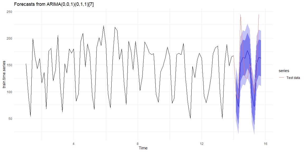
The model selected using AIC coefficient is ARIMA(0, 0, 1) with a seasonal component (0, 1, 1) with frequency 7. The residual plots (on the training data) show that the errors are normally distributed and look like random noise.
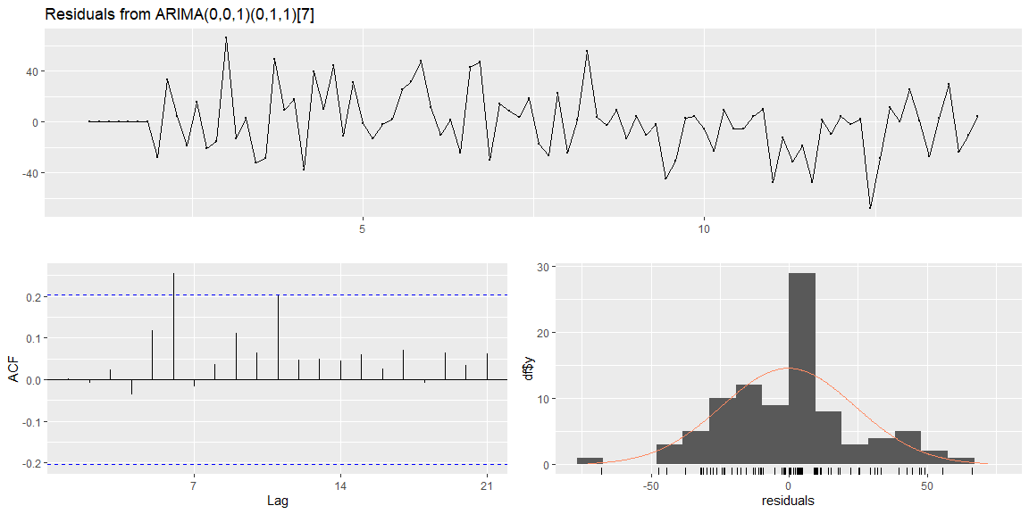
##
##  Ljung-Box test
##
## data:  Residuals from ARIMA(0,0,1)(0,1,1)[7]
## Q* = 15.185, df = 12, p-value = 0.2315
##
## Model df: 2.   Total lags used: 14
Holts Winter model
The Holt-Winters model has three components, level (\(\alpha\)), trend (\(\beta\)) and seasonality (\(\gamma\). In each of these components, there can be additive, multiplicative or no effects. Assuming that the series only has seasonal component, the below plots use additive, multiplicative and damped-multiplicative methods for prediction.
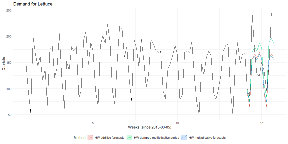 The accuracy of the three models are
## [1] "Aditive Model"
##                 ME  RMSE  MAE   MPE  MAPE MASE ACF1
## Training set -1.35 22.94 18.3 -3.66 14.01 0.69 0.08
## [1] "Multiplicative Model"
##                 ME  RMSE   MAE   MPE  MAPE MASE ACF1
## Training set -1.45 22.96 18.35 -4.37 14.33  0.7 0.08
## [1] "Damped multiplicative Model"
##                ME  RMSE   MAE   MPE  MAPE MASE ACF1
## Training set 0.76 22.67 18.46 -2.13 14.06  0.7 0.12
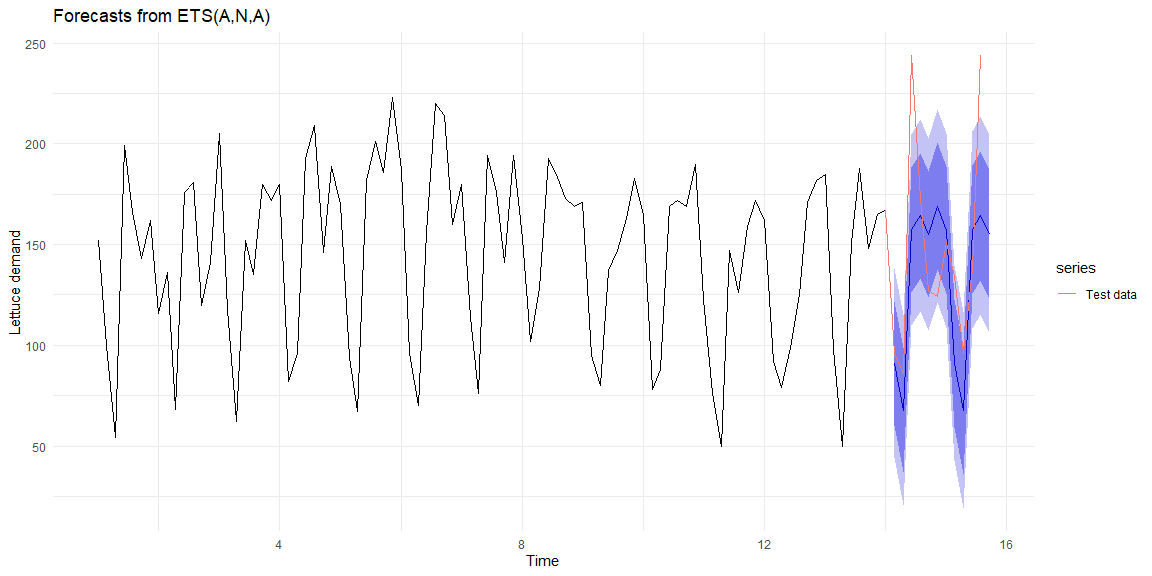
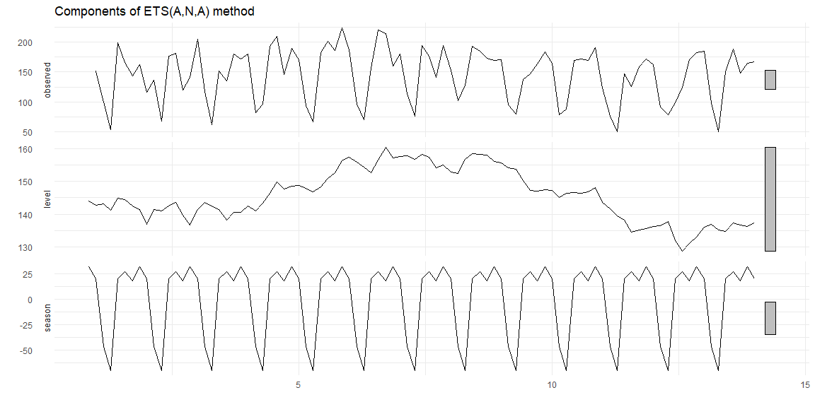
Estimating ETS models
Estimating the \(\alpha, \beta\) and \(\gamma\) parameters by minimizing the sum of squared errors, we get that the additive error type, No trend and additive seasonality.
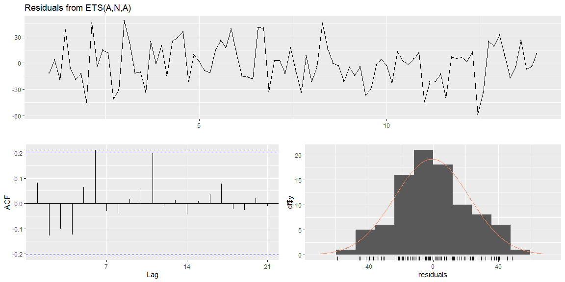
## ETS(A,N,A)
##
## Call:
##  ets(y = train.time.series, model = "ZZZ")
##
##   Smoothing parameters:
##     alpha = 0.0967
##     gamma = 1e-04
##
##   Initial states:
##     l = 143.9203
##     s = 31.7796 17.6211 26.946 20.0456 -69.8942 -46.3021
##            19.804
##
##   sigma:  23.9411
##
##      AIC     AICc      BIC
## 1010.843 1013.560 1036.061
##
## Training set error measures:
##                      ME     RMSE      MAE       MPE     MAPE      MASE
## Training set -0.7342076 22.73998 18.15336 -3.504596 13.98764 0.6891627
##                    ACF1
## Training set 0.08178856
 The residuals (on the training data) are normally distributed and look like random noise.
##
##  Ljung-Box test
##
## data:  Residuals from ETS(A,N,A)
## Q* = 14.79, df = 5, p-value = 0.0113
##
## Model df: 9.   Total lags used: 14
## NULL
Comparison between SARIMA and ETS
The accuracy metrics on the test data for both the models are show below
| ME | RMSE | MAE | MPE | MAPE | MASE | ACF1 | Theil.s.U | |
|---|---|---|---|---|---|---|---|---|
| Holt-Winters Train | -0.73 | 22.74 | 18.15 | -3.50 | 13.99 | 0.69 | 0.08 | NA |
| Holt-Winters Test | 15.54 | 42.83 | 33.50 | 7.71 | 21.65 | 1.27 | 0.06 | 0.62 |
| SARIMA Train | -0.32 | 24.02 | 17.55 | -2.83 | 13.15 | 0.67 | 0.00 | NA |
| SARIMA Test | 13.02 | 44.40 | 34.28 | 5.28 | 21.71 | 1.30 | 0.12 | 0.64 |
Holts-Winter has lower error rate (RMSE, MAE) than SARIMA. Therefore, Holts-winter is the better model.
References
- Forecasting Principles and practice by Rob J Hyndman and George Athanasopoulos
- Blogpost: Stationary tests by Achyuthuni Sri Harsha
- Blogpost: ARIMA by Achyuthuni Sri Harsha
- GitHub code samples by HarshaAsh
- Projects on www.andreasgeorgopoulos.com by Andreas Georgopoulos
- Class notes, Jiahua Wu, Logistics and Supply-Chain Analytics, MSc Business analytics, Imperial College London, Class 2020-22