Probability (R)
Why is probability important
One of the fundamental topics of data science is probability. This is because, in the real world, there are always random effects that cause randomness in even the most predictable events. Randomness is found in daily life to research conducted to business applications we encounter. Probability is a field which provides us with tools to fight against uncertainty and is, therefore, the backbone of statistics, econometrics, game theory and machine learning.
Elements of the probabilistic model
Let us take an experiment where the potential outcomes are \(\omega_1, \omega_2,...\).
For example, if we roll a six-sided die, the outcomes are \(\omega_1 = 1, \omega_2 = 2, \omega_3 = 3, \omega_4 = 4, \omega_5 = 5, \omega_6 = 6\). This set of all outcomes is called a sample space and is denoted by \(\Omega\). A subset of the sample space is called an event. For example, getting 3 or 4 in a six-headed die roll is an event.
Laws of probability
Which event is more likely to occur and which event is less likely to occur. This is explained by using a probability function P(A). There are four laws of probability:
1. \(0 \leq P(A) \leq 1\): The probability of an event is between 0 and 100%.
2. \(P(\Omega) = 1\): the probability of the sample space is 1.
3. If event A and event B are disjoint, then \(P(A \cup B) = P(A) + P(B)\).
4. If events \(A_i\) are pairwise disjoint events, i.e. \(A_i \cap A_j = \phi\), then \(P(\cup_{i=1}^{\infty}A_i) = \sum_{i=0}^\infty P(A_i)\)
Any probability function that satisfies these three axioms are considered to be a valid probability function.
Some properties that can be derived from these axioms are:
1. \(P(A^C) = 1-P(A)\)
2. \(P(A \cap B) = P(A) + P(B) - P(A \cup B)\)
3. If \(A \subset B\) then \(P(A) \leq P(B)\)
4. If \(P(A \cap B) = P(A)P(B)\), then A and B are independent
Conditional probability
Let A and B be two events from the same sample space. The conditional probability of A given B is the probability of A happening if B has already taken place. This is given by \(P(A|B) = \frac{P(A \cap B)}{P(B)}\)
From the above, we can get the following:
1. \(P(A \cap B) = P(B)\times P(A|B) = P(A)\times P(B|A)\)
2. \(P(A) = \sum_{i=1}^n P(A|B_i)\times P(B_i)\) where \(B_i\) form a partition of the sample space. This is called as the formula of total probability
Bayes theorem
If A and B are two events where P(A)>0, then
\(P(A | B) = \frac{P(B|A)P(A)}{\sum_{i=1}^n P(B|A_i)\times P(A_i)}\)
where \(A_j\)'s form a partition of the sample space \(\cup_{i=1}^{\infty}A_i = \Omega\) and for \(i\neq j, A_i \neq A_j\)
Random Variables
Random variables will help us understand the probability distributions. A random variable maps the outcomes from an experiment from the sample space to a numerical quantity. For example, if we flip a coin four times, we can get the following outcomes with H for heads and T for Tails: HTHT, HHTT, HHHT, TTTH, TTTT etc. if we take a variable that measures the number of heads in the series, we get a mapping like: HTHT - 2; HHTT - 2; HHHT - 3; TTTH - 1; TTTT - 0 and so on. The randomness of a random variable is attached to the event, and not the experiment. Random variables are this mapping which maps the outcomes of the experiment to numerical quantities. There are two types of random variables, discrete and continuous random variables.
The range of a discrete random variable contains a finite or countably infinite sequence of values. Some examples are:
1. No of heads in 10 coin flips: finite
2. The number of flips of a coin until heads appear: countable infinite
Continuous random variables have their range as an interval of real numbers which can be finite or infinite. An example would be the time until the next customer arrives in a store.
Distribution functions
Distribution functions are used to characterise the behaviour of random variables, like the mean, standard deviation and probabilities. There are two types of distribution functions, probability distribution functions and cumulative distribution functions.
For discrete random variables, we use probability mass function, which is the probability that a random variable will take a specific value. For continuous random variables, the probability of a random variable will be in an interval is arrived by integrating the probability density function.
The *cumulative distribution functions depict the variable will take the value less than equal to the range.
Two random variables \(Y_1\) and \(Y_2\) are said to be independent of each other if \(P(Y_1 \in A, Y_2 \in B) = P(Y_1 \in A)\times P(Y_2 \in B)\)
Discrete random variables
For discrete random variables, the PMF and CDF are defined as follows:
$$ PMF = p_X(x) := P(X = x) $$
$$ CMF = F_X(x) := P(X\leq x) $$
The mean and variance of discrete random variables
Let X be a random variable with range {\(x_1, x_2, ...\)}. The mean and variance of a random variable are given by:
Expected value (Mean): \(E[X] := \sum_{i=1}^n x_i \times P(X=x_i)\)
Variance: \(Var(X) := E[(X-E[X])^2] = E[X^2]-E[X]^2\)
Standard Deviation \(SD(X) = \sqrt{Var(X)}\)
If two events X and Y are independent, then
1. E[XY] = E[X]E[Y]
2. \(Var(aX+bY) = a^2Var(X) + b^2 Var(Y)\)
Bernoulli distribution
Imagine an experiment that can have two outcomes, success or failure but not both. We call such an experiment as a Bernoulli trial. Consider the random variable X, which assigns 1 when we have success and 0 when we have a failure. If the probability of success is 'p', then the Probability mass function is given by:
\(P(X=x)=\left\{ \begin{array}{ll} p \qquad x=1\\ 1-p \quad x=0 \end{array} \right.\)
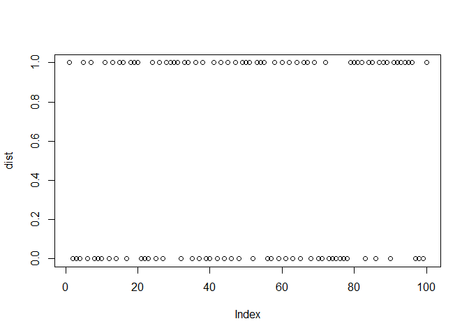
Consider flipping a coin which has a probability of heads as 60%(probability of success) 100 times. Below is a simulation of the same:
dist <- rbinom(100, 1, 0.6)
plot(dist)
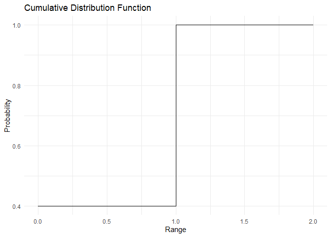
The PMF and CDF of Bernoulli distribution are as shown:
range <- c(0,1)
pmf <- dbinom(x=range, size = 1,prob = 0.6)
cdf <- pbinom(q = range, size = 1, prob = 0.6)
plot_pmf(pmf,range)

plot_cdf(cdf, range)
The mean and variance of the Bernoulli distribution is \(E[X] = p\) and \(Var(X) = p\times q\) This can be verified using the below code
mean(dist)
## [1] 0.54
var(dist)
## [1] 0.2509091
Binomial distribution
Imagine an experiment where we are repeating independent Bernoulli trails n times. Then we can characterise this distribution using only two parameters, the success probability p and the number of trails n. If we have r successes out of n trials, we represent the probability of that event happening using a binomial distribution. The PMF of the binomial distribution is given as
\(P(X=x)=(^nc_r)\times p^r\times q^{n-r}\)
A binomial random variable is the sum of n Bernoulli distributions.
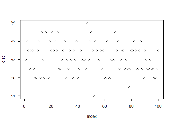
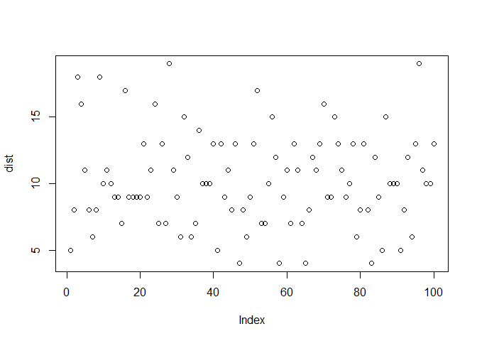
Consider flipping a coin 10 times which has a probability of heads as 60%(probability of success). For the range 0 to 10, the total number of heads in 10 flips is simulated below:
dist <- rbinom(100, 10, 0.6)
plot(dist)
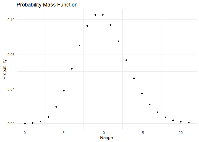
The PMF and CDF of bernoulli distribution are as shown:
range <- c(0,1,2,3,4,5,6,7,8,9,10)
pmf <- dbinom(x=range, size = 10,prob = 0.6)
cdf <- pbinom(q = range, size = 10, prob = 0.6)
plot_pmf(pmf,range)
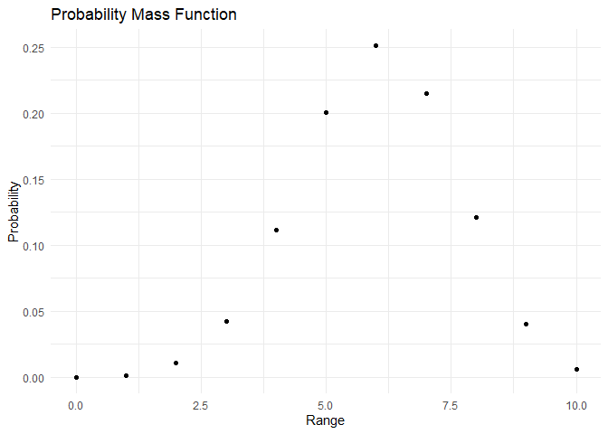
plot_cdf(cdf, range)
The mean and variance of the binomial distribution are \(E[X] = np\) and \(Var[X] = npq\) This can be derived as shown below and verified using the below code:
Derivations:
\(E[X] = E[Z_1 + Z_2 + ...] = E[Z_1] + E[Z_2] +E[Z_3] + ...E[Z_n] = np\)
where \(Z_1, Z_2..Z_n\) are Bernoulli events which constitute the binomial distribution.
\(Var[x] = Var[Z_1 + Z_2 + ...] = Var[Z_1] + Var[Z_2] +Var[Z_3] + ...Var[Z_n] = npq\) as \(Z_1, Z_2..Z_n\) are independent.
The same can also be verified by taking the mean and variance of the sample data:
mean(dist)
## [1] 6.11
var(dist)
## [1] 2.523131
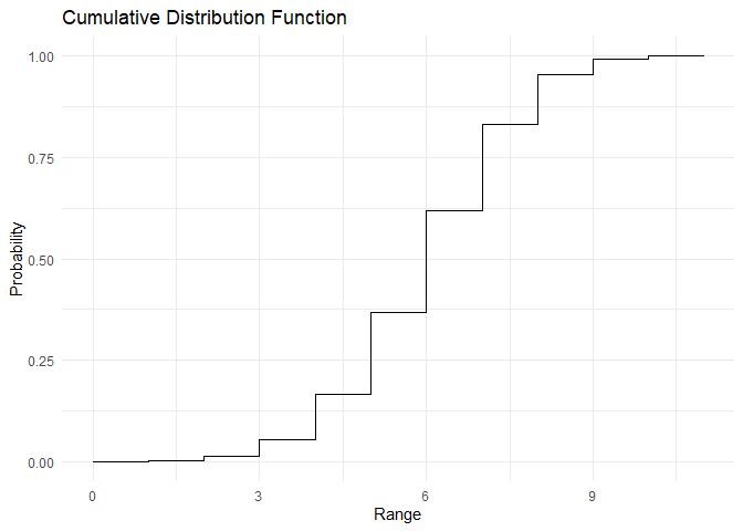
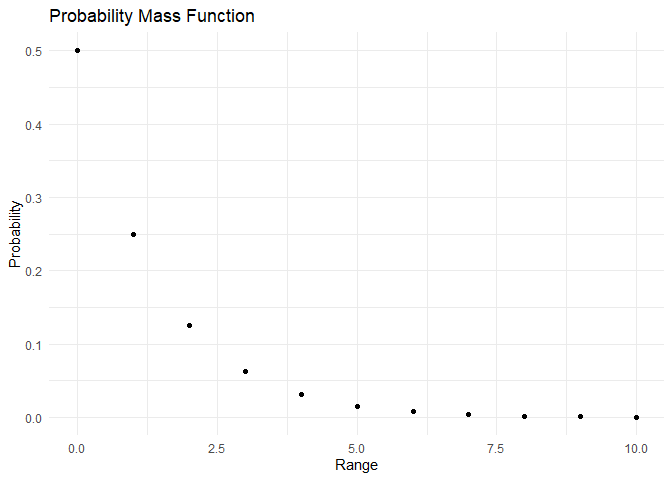
Geometric distribution
Imagine an experiment where we are repeating independent Bernoulli trails n times. We can characterise this distribution using only two parameters, the success probability p and the number of trails n. Consider the event where we get the first success after n failures. The distribution associated with this event is the geometric distribution. The PMF of the binomial distribution is given as
\(P(X=x)=p\times (1-p)^{r}\)
The range of this function is all Real Values from 0,1,2,3,4,...
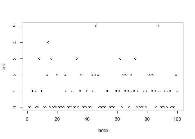
Consider flipping a coin unitil we get heads, where the probability of heads is 50%(probability of success). For the range 0 to 10, the probability of n failures until the first heads is given by:
dist <- rgeom(100, 0.5)
plot(dist)
The PMF and CDF of Geometric distribution are as shown:
range <- c(0,1,2,3,4,5,6,7,8,9,10)
pmf <- dgeom(x=range, prob = 0.5)
cdf <- pgeom(q = range,prob = 0.5)
plot_pmf(pmf,range)
plot_cdf(cdf, range)
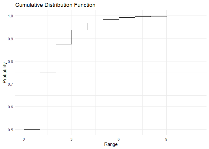
The mean and variance of the geometric distribution are \(E[X] = \frac{q}{p}\) and \(Var[X] = \frac{q}{p^2}\) This can be derived as shown below and verified using the below code:
Derivations:
\(E[X] = 0p+1qp+2q^2p+3q^3p+..=qp(1+2q+3q^2+..) = qp\frac{1}{(1-q)^2} = q/p\)
\(Var[x] = E[X^2]-E[X]^2 = (0p+1qp+4q^2p+9q^3p+..) -(\frac{q}{p})^2 = \frac{q}{p^2}\)
The same can also be verified by taking the mean and variance of the sample data:
mean(dist)
## [1] 0.86
var(dist)
## [1] 1.232727
Poisson distribution
The Poisson distribution is used when we are counting the number of successes in an interval of time. Usually, in these situations, the probability of an event occurring at a particular time is small. For example, we might be interested in counting the number of customers that arrive in a bus stand in a period of time. This random variable might follow a Poisson distribution as the probability of success; someone coming to the bus stand at any tick of time is small. Only one parameter is used to define the Poisson distribution, i.e. \(\lambda\), which is the average rate of arrivals we are interested in. The PMF is defined as
$$ P(X=x)= \frac{\lambdaxe $$ The range of this function is all Real Values from 0,1,2,3,4,... }}{x!
For a Poisson distribution of \(\lambda =10\), we have
dist <- rpois(100, 10)
plot(dist)
The PMF and CDF of Poisson distribution are as shown:
range <- c(0,1,2,3,4,5,6,7,8,9,10, 11, 12, 13, 14, 15, 16, 17, 18, 19, 20, 21)
pmf <- dpois(x=range, lambda = 10)
cdf <- ppois(q = range, lambda = 10)
plot_pmf(pmf,range)
plot_cdf(cdf, range)

The mean and variance of the Poisson distribution are \(E[X] = \lambda\) and \(Var[X] = \lambda\) This can be derived as shown below and verified using the below code:
Derivations:
\(E[X] = \sum x\frac{\lambda^xe^{-\lambda}}{x!} = \lambda \sum\frac{\lambda^{x-1}e^{-1}}{(x-1)!} = \lambda\)
The same can also be verified by taking the mean and variance of the sample data:
mean(dist)
## [1] 10.24
var(dist)
## [1] 12.28525
Continuous random variables
Unlike discrete random variables, continuous random variables can take all real values in an interval which can be finite or infinite. A continuous random variable X has a probability density function \(f_X(X)\). PDF is different from PMF while its usage in calculating the probability of an event is similar. For instance, the probability of an event A is calculated by summing the probabilities of each discrete variable(PMF), while we integrate the probabilities for all the outcomes for continuous variables(PDF). Similarly, for CDF, we integrate from \(-\infty\) to x.
\(PDF:= f_X(x)\)
\(P(X\in A) = \int_A f_X(y) dy\)
\(CDF:= F_X(x) = \int_{-\infty}^{x} f_x(y) dy\)
Therefore PDF and CDF are lated by \(\frac{d}{dx}F(X) = f(x)\) and \(P(X \in (x+\epsilon, x-\epsilon)) = 2\epsilon \times f(x)\).
Uniform distribution
The uniform distribution is used when we do not have the underlying distribution at hand. We make a simplifying assumption that every element in our range has the same probability of occurring. The PDF of a uniform distribution is given by:
\(PDF:= f(x) = \frac{1}{b-a}, \, x \in (a,b)\)
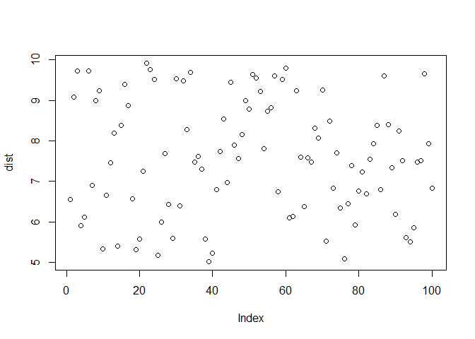
We need two parameters to characterise a uniform distribution, which is a and b. The distribution is as shown:
dist <- runif(n = 100, min = 5, max = 10)
plot(dist)
The PDF and CDF are plotted below:
range <- 1:150/10
pdf <- dunif(x=range, min=5, max=10)
cdf <- punif(q = range, min=5, max=10)
plot_pdf(pdf,range)
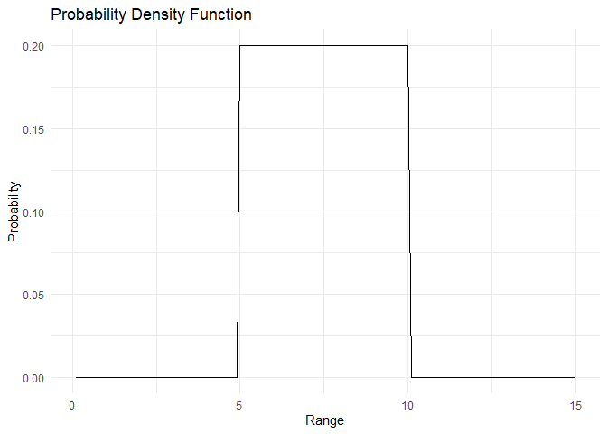
plot_cdf_continuous(cdf, range)
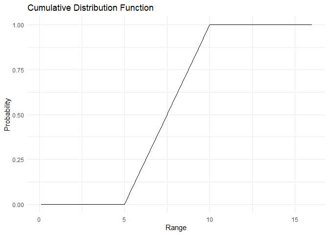
For the uniform distribution, the mean is \(E[X]=\frac{a+b}{2}\) and variance is \(Var[X] = \frac{(a-b)^2}{12}\). This can be proven using:
\(E[X] = \int_a^bx\times\frac{1}{b-a}dx = \frac{a+b}{2}\)
\(Var[X] = E[X^2] - E[X]^2 = \int_a^b x^2\times \frac{1}{b-a}dx - (\frac{a+b}{2})^2 = \frac{(b^3-a^3)}{3(b-a)}- \frac{(a+b)^2}{4} = \frac{a^2+b^2+ab}{4}-\frac{(a+b)^2}{4} = \frac{(a-b)^2}{12}\)
The same can also be verified by taking the mean and variance of the sample data:
mean(dist)
## [1] 7.592581
var(dist)
## [1] 2.017721
Exponential distribution
In the geometric distribution, we looked at the probability of first success happening after n failures. In the exponential distribution, we look at the time taken until which an event occurs, or time elapsed between events. Only one parameter is sufficient to describe an exponential distribution, \(\lambda\) which describes the successes per unit time. The PDF of an exponential distribution is given as:
\(PDF:= f(x) = \lambda\times e^{-\lambda x}\)
The CDF can be derived as
\(CDF = P(X<x) = F(X) = \int_0^x \lambda\times e^{-\lambda y} dy = 1-e^{-\lambda x}\)
Therefore 1-CDF can be written as
\(P(X>x) = e^{-\lambda x}\)
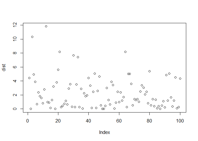
The intervel \(x>0\) and \(\lambda>0\). The distribution if an event happens on an average once every two minutes is as shown:
dist <- rexp(n = 100,rate = 0.5)
plot(dist)
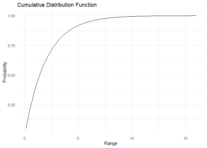
The PDF and CDF are plotted below:
range <- 1:150/10
pdf <- dexp(x=range, rate= 0.5)
cdf <- pexp(q = range, rate = 0.5)
plot_pdf(pdf,range)
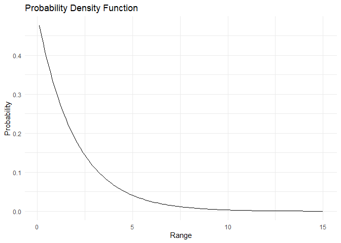
plot_cdf_continuous(cdf, range)
For the exponential distribution, the mean is \(E[X]=\frac{1}{\lambda}\) and variance is \(Var[X] = \frac{1}{\lambda^2}\).
The same can also be verified by taking the mean and variance of the sample data:
mean(dist)
## [1] 2.309103
var(dist)
## [1] 5.504272
Normal distribution
The normal distribution is the most famous continuous distribution. It has a unique bell-shaped curve. Randomness generally presents as a normal distribution. It is widespread in nature. Two parameters define a normal distribution, its mean \(\mu\) and standard deviation \(\sigma\).
\(PDF:= f(x) = \frac{1}{2\pi \sigma^2}e^{-\frac{(x-\mu)^2}{2\sigma^2}}\)
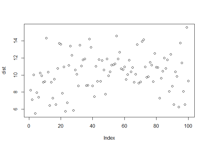
The distribution with mean 10 and standard deviation 2 is as shown:
dist <- rnorm(n = 100,mean = 10, sd = 2)
plot(dist)
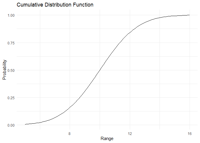
The PDF and CDF are plotted below:
range <- 50:150/10
pdf <- dnorm(x=range, mean = 10, sd = 2)
cdf <- pnorm(q = range, mean = 10, sd = 2)
plot_pdf(pdf,range)

plot_cdf_continuous(cdf, range)
References
- Blitzstein, JK and Hwang, J (2014). Introduction to Probability. CRC Press LLC
- Dinesh Kumar (2019). Business Analytics: the science of Data-Driven Decision Making