Linear Regression (R)

Introduction¶

Regression problems are an important category of problems in analytics in which the response variable $Y$ takes a continuous value. For example, a regression goal is predicting housing prices in an area. In this blog post, I will attempt to solve a supervised regression problem using the famous Boston housing price data set. Other than location and square footage, a house value is determined by various other factors.
The data used in this blog is taken from Kaggle. It originates from the UCI Machine Learning Repository. The Boston housing data was collected in 1978 and each of the 506 entries represent aggregated data about 14 features for homes from various suburbs in Boston, Massachusetts.
The data frame contains the following columns:
crim: per capita crime rate by town.
zn: proportion of residential land zoned for lots over 25,000 sq.ft.
indus: proportion of non-retail business acres per town.
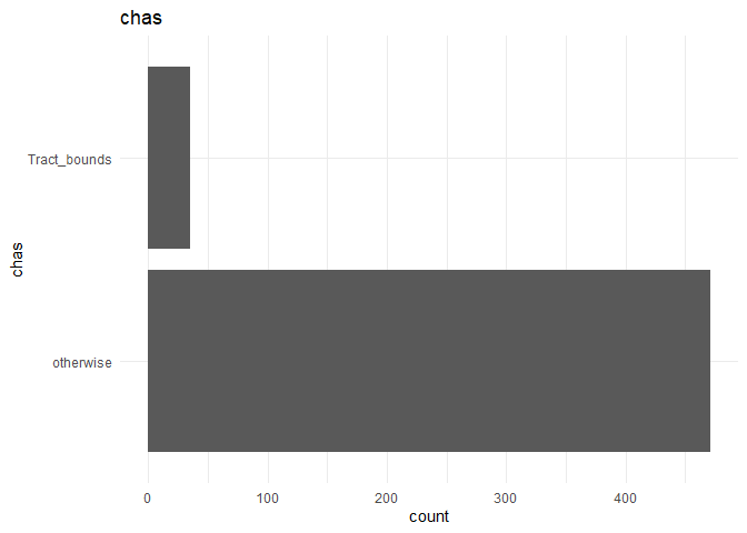
chas: Charles River categorical variable (tract bounds or otherwise).
nox: nitrogen oxides concentration (parts per 10 million).
rm: average number of rooms per dwelling.
age: proportion of owner-occupied units built prior to 1940.
dis: weighted mean of distances to five Boston employment centres.
rad: index of accessibility to radial highways.
tax: full-value property-tax rate per $10,000.
ptratio: pupil-teacher ratio by town.
black: racial discrimination factor.
lstat: lower status of the population (percent)

The target variable is
medv: median value of owner-occupied homes in $1000s.

In particular, in this blog I want to use multiple linear regression for the analysis. A sample of the data is given below:

Sample data
crim	zn	indus	chas	nox	rm	age	dis	rad	tax	ptratio	black	lstat	medv
2.92400	0.0	19.58	otherwise	0.6050	6.101	93.0	2.2834	5	403	14.7	240.16	9.81	25.0
0.12816	12.5	6.07	otherwise	0.4090	5.885	33.0	6.4980	4	345	18.9	396.90	8.79	20.9
0.08244	30.0	4.93	otherwise	0.4280	6.481	18.5	6.1899	6	300	16.6	379.41	6.36	23.7
0.06588	0.0	2.46	otherwise	0.4880	7.765	83.3	2.7410	3	193	17.8	395.56	7.56	39.8
0.02009	95.0	2.68	otherwise	0.4161	8.034	31.9	5.1180	4	224	14.7	390.55	2.88	50.0

The summary statistics for the data is:

##       crim                zn             indus           chas          
##  Min.   : 0.00632   Min.   :  0.00   Min.   : 0.46   Length:506        
##  1st Qu.: 0.08205   1st Qu.:  0.00   1st Qu.: 5.19   Class :character  
##  Median : 0.25651   Median :  0.00   Median : 9.69   Mode  :character  
##  Mean   : 3.61352   Mean   : 11.36   Mean   :11.14                     
##  3rd Qu.: 3.67708   3rd Qu.: 12.50   3rd Qu.:18.10                     
##  Max.   :88.97620   Max.   :100.00   Max.   :27.74                     
##       nox               rm             age              dis        
##  Min.   :0.3850   Min.   :3.561   Min.   :  2.90   Min.   : 1.130  
##  1st Qu.:0.4490   1st Qu.:5.886   1st Qu.: 45.02   1st Qu.: 2.100  
##  Median :0.5380   Median :6.208   Median : 77.50   Median : 3.207  
##  Mean   :0.5547   Mean   :6.285   Mean   : 68.57   Mean   : 3.795  
##  3rd Qu.:0.6240   3rd Qu.:6.623   3rd Qu.: 94.08   3rd Qu.: 5.188  
##  Max.   :0.8710   Max.   :8.780   Max.   :100.00   Max.   :12.127  
##       rad              tax           ptratio          black       
##  Min.   : 1.000   Min.   :187.0   Min.   :12.60   Min.   :  0.32  
##  1st Qu.: 4.000   1st Qu.:279.0   1st Qu.:17.40   1st Qu.:375.38  
##  Median : 5.000   Median :330.0   Median :19.05   Median :391.44  
##  Mean   : 9.549   Mean   :408.2   Mean   :18.46   Mean   :356.67  
##  3rd Qu.:24.000   3rd Qu.:666.0   3rd Qu.:20.20   3rd Qu.:396.23  
##  Max.   :24.000   Max.   :711.0   Max.   :22.00   Max.   :396.90  
##      lstat            medv      
##  Min.   : 1.73   Min.   : 5.00  
##  1st Qu.: 6.95   1st Qu.:17.02  
##  Median :11.36   Median :21.20  
##  Mean   :12.65   Mean   :22.53  
##  3rd Qu.:16.95   3rd Qu.:25.00  
##  Max.   :37.97   Max.   :50.00

Data Cleaning and EDA¶

Zero and Near Zero Variance features do not explain any variance in the predictor variable.

Zero and near zero variance
	freqRatio	percentUnique	zeroVar	nzv
crim	1.000000	99.6047431	FALSE	FALSE
zn	17.714286	5.1383399	FALSE	FALSE
indus	4.400000	15.0197628	FALSE	FALSE
chas	13.457143	0.3952569	FALSE	FALSE
nox	1.277778	16.0079051	FALSE	FALSE
rm	1.000000	88.1422925	FALSE	FALSE
age	10.750000	70.3557312	FALSE	FALSE
dis	1.250000	81.4229249	FALSE	FALSE
rad	1.147826	1.7786561	FALSE	FALSE
tax	3.300000	13.0434783	FALSE	FALSE
ptratio	4.117647	9.0909091	FALSE	FALSE
black	40.333333	70.5533597	FALSE	FALSE
lstat	1.000000	89.9209486	FALSE	FALSE
medv	2.000000	45.2569170	FALSE	FALSE

There are no near zero or zero variance columns

Similarly, I can check for linearly dependent columns among the continuous variables.

## $linearCombos
## list()
## 
## $remove
## NULL

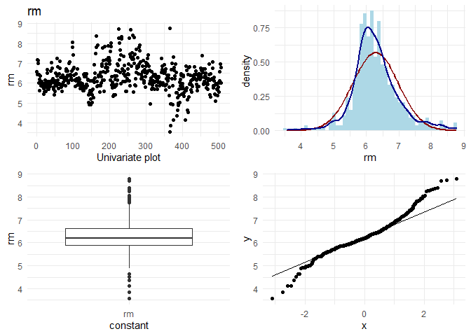
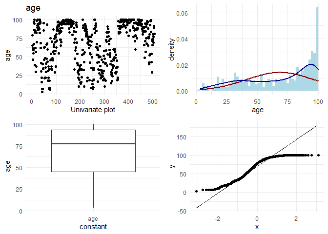
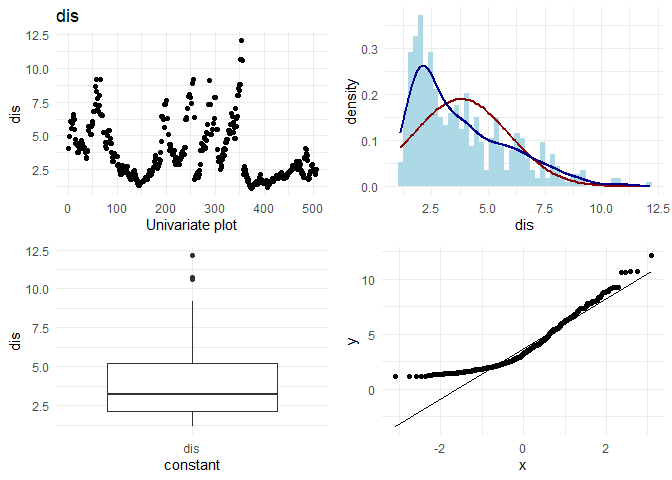
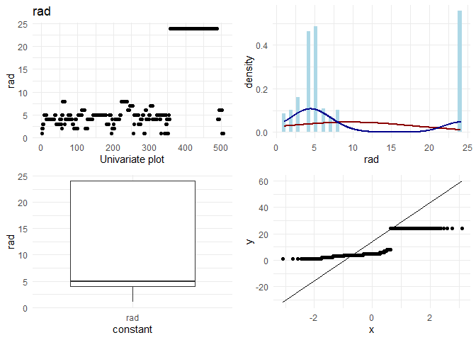
There are no linearly dependent columns.

Uni-variate analysis¶

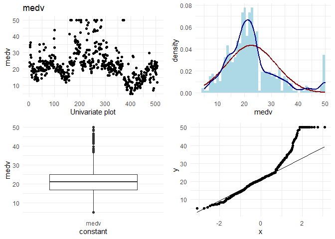
Now, I want to do some basic EDA on each column. On each continuous column, I want to visually check the following:
1. Variation in the column
2. Its distribution
3. Any outliers
4. q-q plot with normal distribution

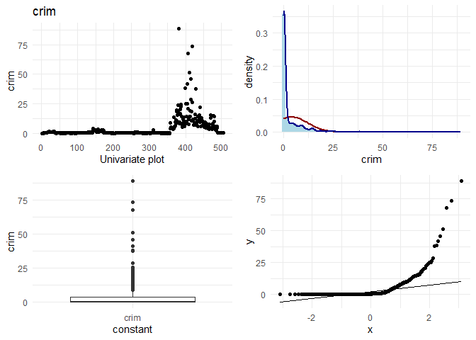
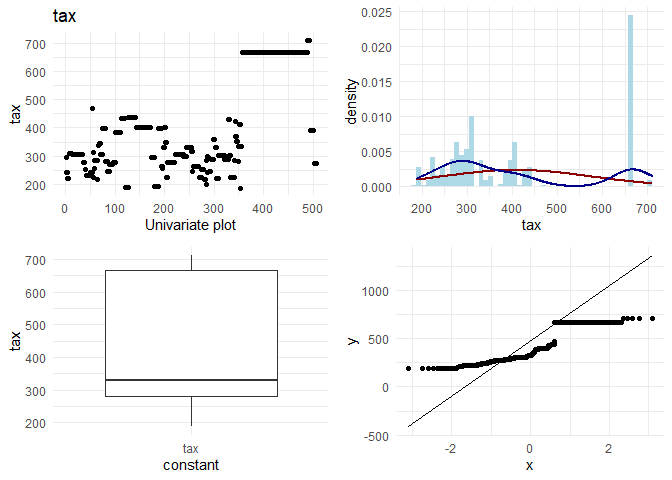
## [1] "Univariate plots for crim"

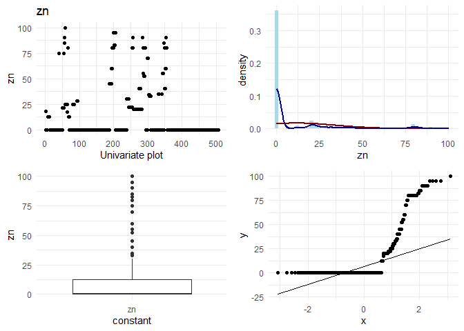
## [1] "Univariate plots for zn"

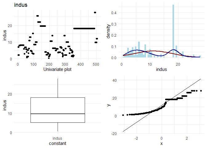
## [1] "Univariate plots for indus"

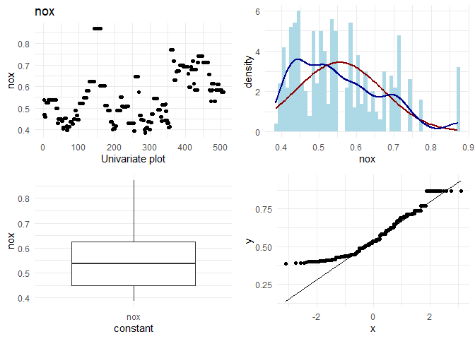
## [1] "Univariate plots for nox"

## [1] "Univariate plots for rm"

## [1] "Univariate plots for age"

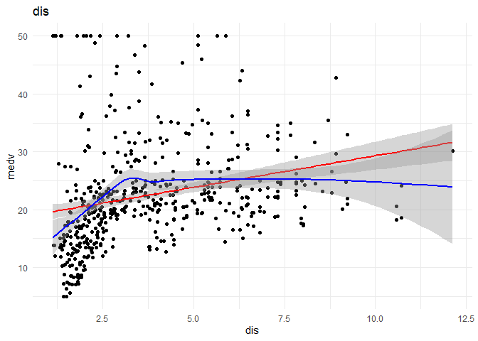
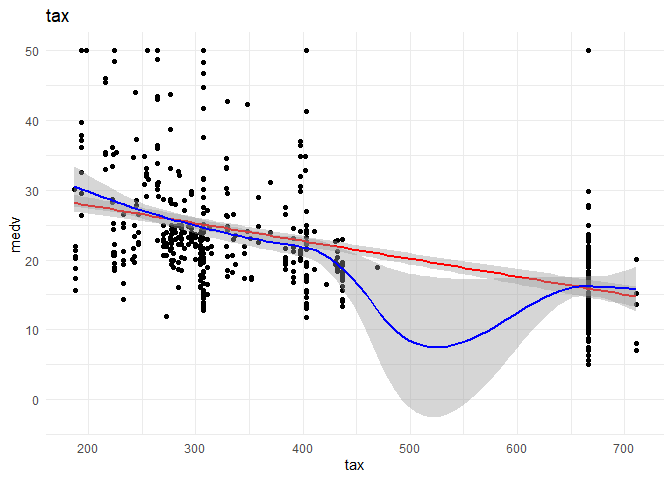
## [1] "Univariate plots for dis"

## [1] "Univariate plots for rad"

## [1] "Univariate plots for tax"

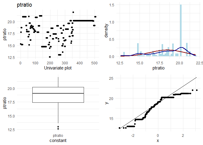
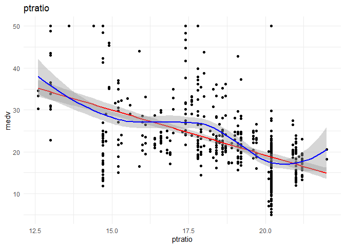
## [1] "Univariate plots for ptratio"

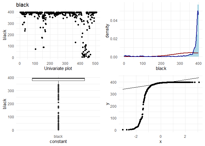
## [1] "Univariate plots for black"

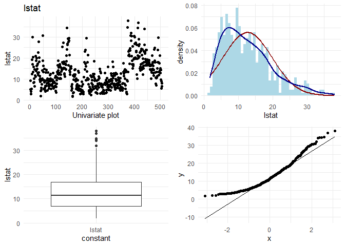
## [1] "Univariate plots for lstat"

## [1] "Univariate plots for medv"

For categorical variables, I want to look at the frequencies.

Observations:
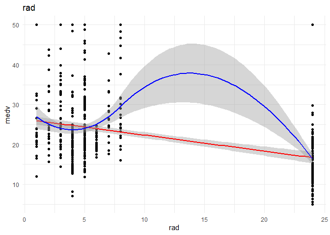
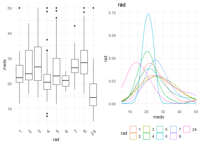
1. If I look at rad and tax, I observe that there seem to be two categories. Houses having rad < 10 follow a normal distribution, and there are some houses with rad = 24. As rad is an index, it could also be thought of as a categorical variable instead of a continuous variable.
2. For data points with rad= 25, the behaviour in location based features looks different. For example indus, tax and ptratio have a different slope at the same points where the rad is 24. (observation for variation plots(top left plots))

Therefore, I am tempted to group the houses which have rad = 24 into one category, and create interaction variables of that column with rad, indus, ptratio and tax. The new variable is called rad_cat. Also, I would like to convert rad itself to categorical and see if it can explain better than continuous variable.
Additionally, from researching on the internet, I found that the cost might have a different slope with the number of bedrooms for different class of people. So, I want to visualize that interaction variable also.

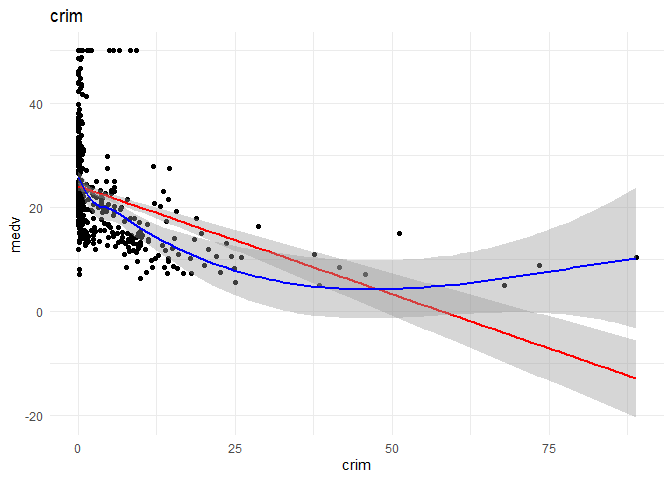
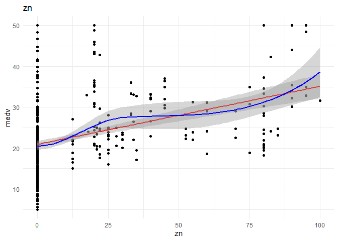
Bi variate analysis¶

I want to understand the relationship of each continuous variable with the $y$ variable. I will achieve that by doing the following:
1. A scatter plot to look at the relationship between the $x$ and the $y$ variables.
2. Draw a linear regression line and a smoothed means line to understand the curve fit.
3. Predict using Linear regression using the variable alone to observe the increase in R-squared.

## 
## Call:
## lm(formula = .outcome ~ ., data = dat)
## 
## Residuals:
##     Min      1Q  Median      3Q     Max 
## -15.816  -5.455  -1.970   2.633  29.615 
## 
## Coefficients:
##             Estimate Std. Error t value Pr(>|t|)    
## (Intercept) 23.99736    0.45955  52.220  < 2e-16 ***
## crim        -0.39123    0.04855  -8.059 8.75e-15 ***
## ---
## Signif. codes:  0 '***' 0.001 '**' 0.01 '*' 0.05 '.' 0.1 ' ' 1
## 
## Residual standard error: 8.595 on 405 degrees of freedom
## Multiple R-squared:  0.1382, Adjusted R-squared:  0.1361 
## F-statistic: 64.94 on 1 and 405 DF,  p-value: 8.748e-15
## 
## [1] "----------------------------------------------------------------------------------------------------"

## 
## Call:
## lm(formula = .outcome ~ ., data = dat)
## 
## Residuals:
##      Min       1Q   Median       3Q      Max 
## -15.9353  -5.6853  -0.9847   2.4653  29.0647 
## 
## Coefficients:
##             Estimate Std. Error t value Pr(>|t|)    
## (Intercept) 20.93532    0.48739  42.954  < 2e-16 ***
## zn           0.14247    0.01818   7.835 4.15e-14 ***
## ---
## Signif. codes:  0 '***' 0.001 '**' 0.01 '*' 0.05 '.' 0.1 ' ' 1
## 
## Residual standard error: 8.812 on 405 degrees of freedom
## Multiple R-squared:  0.1316, Adjusted R-squared:  0.1295 
## F-statistic: 61.39 on 1 and 405 DF,  p-value: 4.155e-14
## 
## [1] "----------------------------------------------------------------------------------------------------"

## 
## Call:
## lm(formula = .outcome ~ ., data = dat)
## 
## Residuals:
##     Min      1Q  Median      3Q     Max 
## -12.922  -5.144  -1.631   2.972  33.069 
## 
## Coefficients:
##             Estimate Std. Error t value Pr(>|t|)    
## (Intercept) 30.04045    0.77385   38.82   <2e-16 ***
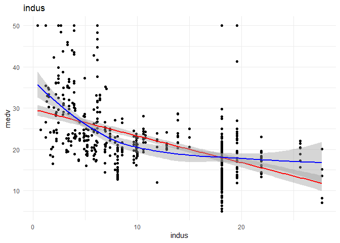
## indus       -0.66951    0.05936  -11.28   <2e-16 ***
## ---
## Signif. codes:  0 '***' 0.001 '**' 0.01 '*' 0.05 '.' 0.1 ' ' 1
## 
## Residual standard error: 8.249 on 405 degrees of freedom
## Multiple R-squared:  0.239,  Adjusted R-squared:  0.2372 
## F-statistic: 127.2 on 1 and 405 DF,  p-value: < 2.2e-16
## 
## [1] "----------------------------------------------------------------------------------------------------"

## 
## Call:
## lm(formula = .outcome ~ ., data = dat)
## 
## Residuals:
##     Min      1Q  Median      3Q     Max 
## -13.688  -5.146  -2.299   2.794  30.643 
## 
## Coefficients:
##             Estimate Std. Error t value Pr(>|t|)    
## (Intercept)   42.020      2.081  20.195   <2e-16 ***
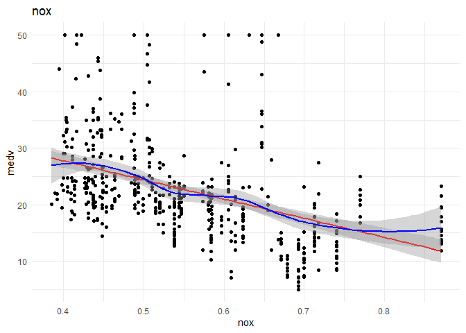
## nox          -35.028      3.680  -9.518   <2e-16 ***
## ---
## Signif. codes:  0 '***' 0.001 '**' 0.01 '*' 0.05 '.' 0.1 ' ' 1
## 
## Residual standard error: 8.548 on 405 degrees of freedom
## Multiple R-squared:  0.1828, Adjusted R-squared:  0.1808 
## F-statistic:  90.6 on 1 and 405 DF,  p-value: < 2.2e-16
## 
## [1] "----------------------------------------------------------------------------------------------------"

## 
## Call:
## lm(formula = .outcome ~ ., data = dat)
## 
## Residuals:
##     Min      1Q  Median      3Q     Max 
## -19.886  -2.551   0.174   3.009  39.729 
## 
## Coefficients:
##             Estimate Std. Error t value Pr(>|t|)    
## (Intercept) -36.6702     2.8680  -12.79   <2e-16 ***
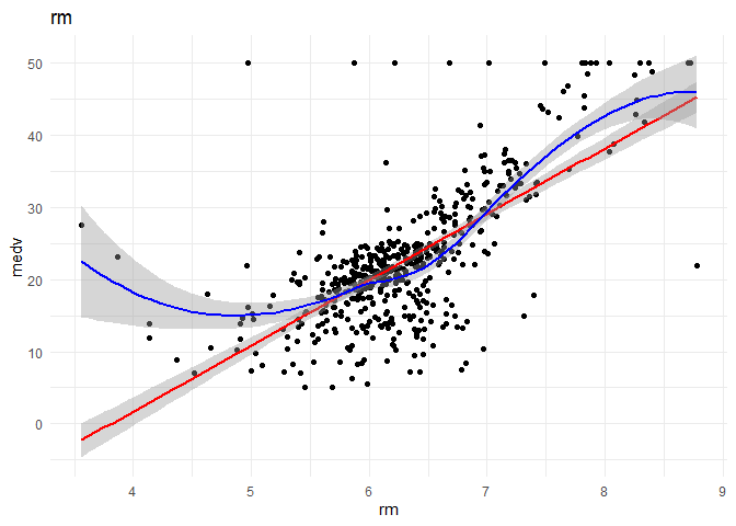
## rm            9.4450     0.4538   20.81   <2e-16 ***
## ---
## Signif. codes:  0 '***' 0.001 '**' 0.01 '*' 0.05 '.' 0.1 ' ' 1
## 
## Residual standard error: 6.574 on 405 degrees of freedom
## Multiple R-squared:  0.5168, Adjusted R-squared:  0.5156 
## F-statistic: 433.1 on 1 and 405 DF,  p-value: < 2.2e-16
## 
## [1] "----------------------------------------------------------------------------------------------------"

## 
## Call:
## lm(formula = .outcome ~ ., data = dat)
## 
## Residuals:
##     Min      1Q  Median      3Q     Max 
## -15.138  -5.266  -2.033   2.333  31.332 
## 
## Coefficients:
##             Estimate Std. Error t value Pr(>|t|)    
## (Intercept)  31.1468     1.1373  27.386  < 2e-16 ***
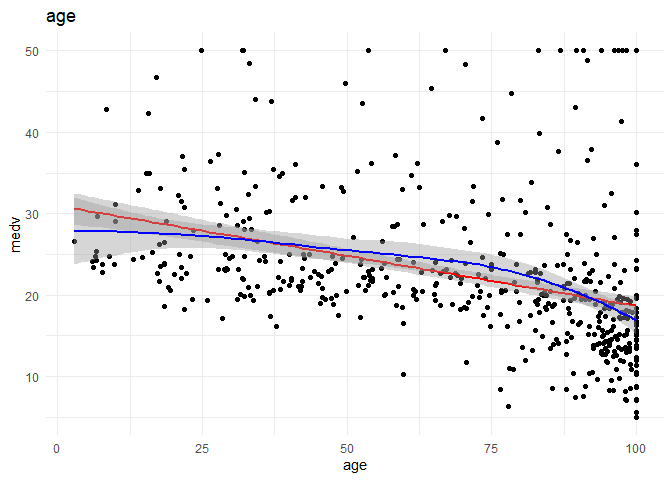
## age          -0.1248     0.0154  -8.104 6.33e-15 ***
## ---
## Signif. codes:  0 '***' 0.001 '**' 0.01 '*' 0.05 '.' 0.1 ' ' 1
## 
## Residual standard error: 8.772 on 405 degrees of freedom
## Multiple R-squared:  0.1395, Adjusted R-squared:  0.1374 
## F-statistic: 65.68 on 1 and 405 DF,  p-value: 6.333e-15
## 
## [1] "----------------------------------------------------------------------------------------------------"

## 
## Call:
## lm(formula = .outcome ~ ., data = dat)
## 
## Residuals:
##     Min      1Q  Median      3Q     Max 
## -15.010  -5.867  -1.968   2.297  30.275 
## 
## Coefficients:
##             Estimate Std. Error t value Pr(>|t|)    
## (Intercept)  18.4243     0.9436  19.526  < 2e-16 ***
## dis           1.1127     0.2188   5.085 5.62e-07 ***
## ---
## Signif. codes:  0 '***' 0.001 '**' 0.01 '*' 0.05 '.' 0.1 ' ' 1
## 
## Residual standard error: 9.168 on 405 degrees of freedom
## Multiple R-squared:  0.06002,    Adjusted R-squared:  0.0577 
## F-statistic: 25.86 on 1 and 405 DF,  p-value: 5.619e-07
## 
## [1] "----------------------------------------------------------------------------------------------------"

## 
## Call:
## lm(formula = .outcome ~ ., data = dat)
## 
## Residuals:
##     Min      1Q  Median      3Q     Max 
## -18.022  -5.310  -2.298   3.375  33.475 
## 
## Coefficients:
##             Estimate Std. Error t value Pr(>|t|)    
## (Intercept)  26.7220     0.6412  41.677   <2e-16 ***
## rad          -0.4249     0.0493  -8.619   <2e-16 ***
## ---
## Signif. codes:  0 '***' 0.001 '**' 0.01 '*' 0.05 '.' 0.1 ' ' 1
## 
## Residual standard error: 8.693 on 405 degrees of freedom
## Multiple R-squared:  0.155,  Adjusted R-squared:  0.1529 
## F-statistic: 74.28 on 1 and 405 DF,  p-value: < 2.2e-16
## 
## [1] "----------------------------------------------------------------------------------------------------"

## 
## Call:
## lm(formula = .outcome ~ ., data = dat)
## 
## Residuals:
##     Min      1Q  Median      3Q     Max 
## -13.039  -5.235  -2.191   3.166  34.209 
## 
## Coefficients:
##              Estimate Std. Error t value Pr(>|t|)    
## (Intercept) 33.707058   1.080289   31.20   <2e-16 ***
## tax         -0.026900   0.002427  -11.09   <2e-16 ***
## ---
## Signif. codes:  0 '***' 0.001 '**' 0.01 '*' 0.05 '.' 0.1 ' ' 1
## 
## Residual standard error: 8.283 on 405 degrees of freedom
## Multiple R-squared:  0.2328, Adjusted R-squared:  0.2309 
## F-statistic: 122.9 on 1 and 405 DF,  p-value: < 2.2e-16
## 
## [1] "----------------------------------------------------------------------------------------------------"

## 
## Call:
## lm(formula = .outcome ~ ., data = dat)
## 
## Residuals:
##      Min       1Q   Median       3Q      Max 
## -19.4897  -4.9434  -0.7651   3.4363  31.2566 
## 
## Coefficients:
##             Estimate Std. Error t value Pr(>|t|)    
## (Intercept)  64.8226     3.4209   18.95   <2e-16 ***
## ptratio      -2.2811     0.1837  -12.42   <2e-16 ***
## ---
## Signif. codes:  0 '***' 0.001 '**' 0.01 '*' 0.05 '.' 0.1 ' ' 1
## 
## Residual standard error: 8.047 on 405 degrees of freedom
## Multiple R-squared:  0.2758, Adjusted R-squared:  0.274 
## F-statistic: 154.2 on 1 and 405 DF,  p-value: < 2.2e-16
## 
## [1] "----------------------------------------------------------------------------------------------------"

## 
## Call:
## lm(formula = .outcome ~ ., data = dat)
## 
## Residuals:
##     Min      1Q  Median      3Q     Max 
## -18.573  -5.028  -1.864   2.874  27.066 
## 
## Coefficients:
##              Estimate Std. Error t value Pr(>|t|)    
## (Intercept) 10.505391   1.785873   5.882 8.47e-09 ***
## black        0.033945   0.004844   7.008 1.02e-11 ***
## ---
## Signif. codes:  0 '***' 0.001 '**' 0.01 '*' 0.05 '.' 0.1 ' ' 1
## 
## Residual standard error: 8.93 on 405 degrees of freedom
## Multiple R-squared:  0.1081, Adjusted R-squared:  0.1059 
## F-statistic: 49.11 on 1 and 405 DF,  p-value: 1.017e-11
## 
## [1] "----------------------------------------------------------------------------------------------------"

## 
## Call:
## lm(formula = .outcome ~ ., data = dat)
## 
## Residuals:
##     Min      1Q  Median      3Q     Max 
## -10.023  -4.173  -1.390   2.172  24.327 
## 
## Coefficients:
##             Estimate Std. Error t value Pr(>|t|)    
## (Intercept) 34.88480    0.63310   55.10   <2e-16 ***
## lstat       -0.96665    0.04336  -22.29   <2e-16 ***
## ---
## Signif. codes:  0 '***' 0.001 '**' 0.01 '*' 0.05 '.' 0.1 ' ' 1
## 
## Residual standard error: 6.336 on 405 degrees of freedom
## Multiple R-squared:  0.551,  Adjusted R-squared:  0.5499 
## F-statistic:   497 on 1 and 405 DF,  p-value: < 2.2e-16
## 
## [1] "----------------------------------------------------------------------------------------------------"

## 
## Call:
## lm(formula = .outcome ~ ., data = dat)
## 
## Residuals:
##     Min      1Q  Median      3Q     Max 
## -10.849  -4.148  -1.339   2.469  24.772 
## 
## Coefficients:
##              Estimate Std. Error t value Pr(>|t|)    
## (Intercept) 36.112064   0.696107   51.88   <2e-16 ***
## rm.lstat    -0.176325   0.008117  -21.72   <2e-16 ***
## ---
## Signif. codes:  0 '***' 0.001 '**' 0.01 '*' 0.05 '.' 0.1 ' ' 1
## 
## Residual standard error: 6.36 on 405 degrees of freedom
## Multiple R-squared:  0.5382, Adjusted R-squared:  0.537 
## F-statistic: 471.9 on 1 and 405 DF,  p-value: < 2.2e-16
## 
## [1] "----------------------------------------------------------------------------------------------------"

Observations:
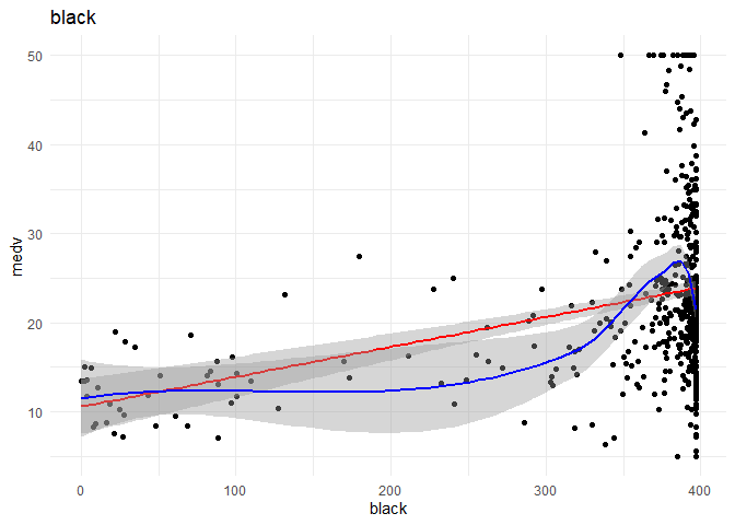
1. Crim and black might have a non-linear relationship with medv, I want further analysis on that front.
2. As thought before rad might be better classified as a categorical variable.
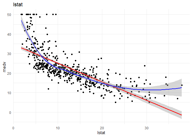
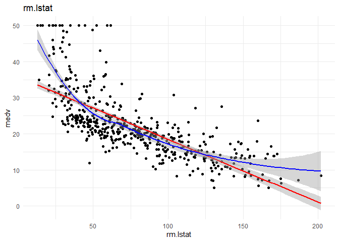
3. lmstat and lm might have a quadratic relationship with medv.

I want to understand the relationship of each categorical variable with the $y$ variable. I will achieve that by doing the following:
1. A box plot showing the difference between variation of y between different classes of the variable.
2. Density plot for each class in the variable to understand the distribution and spread of each class. (If the means were far away from each other and both the classes have small standard deviation, then the variables explainability is more)
3. Predict using Linear regression using the variable alone to observe the increase in R-square

## 
## Call:
## lm(formula = .outcome ~ ., data = dat)
## 
## Residuals:
##     Min      1Q  Median      3Q     Max 
## -17.189  -6.092  -1.389   2.812  27.811 
## 
## Coefficients:
##                  Estimate Std. Error t value Pr(>|t|)    
## (Intercept)       22.1885     0.4766  46.553  < 2e-16 ***
## chasTract_bounds   6.9077     1.8858   3.663 0.000282 ***
## ---
## Signif. codes:  0 '***' 0.001 '**' 0.01 '*' 0.05 '.' 0.1 ' ' 1
## 
## Residual standard error: 9.303 on 405 degrees of freedom
## Multiple R-squared:  0.03207,    Adjusted R-squared:  0.02968 
## F-statistic: 13.42 on 1 and 405 DF,  p-value: 0.0002823
## 
## [1] "----------------------------------------------------------------------------------------------------"

## 
## Call:
## lm(formula = .outcome ~ ., data = dat)
## 
## Residuals:
##     Min      1Q  Median      3Q     Max 
## -14.853  -5.471  -1.853   3.545  33.741 
## 
## Coefficients:
##             Estimate Std. Error t value Pr(>|t|)    
## (Intercept)  25.3692     2.3093  10.986  < 2e-16 ***
## rad2          1.8117     2.9384   0.617 0.537872    
## rad3          2.7756     2.7791   0.999 0.318530    
## rad4         -3.9421     2.4671  -1.598 0.110865    
## rad5          0.9137     2.4638   0.371 0.710934    
## rad6         -4.4587     2.9969  -1.488 0.137609    
## rad7          1.3308     3.2070   0.415 0.678396    
## rad8          5.4837     3.0677   1.788 0.074610 .  
## rad24        -9.1100     2.4443  -3.727 0.000222 ***
## ---
## Signif. codes:  0 '***' 0.001 '**' 0.01 '*' 0.05 '.' 0.1 ' ' 1
## 
## Residual standard error: 8.326 on 398 degrees of freedom
## Multiple R-squared:  0.2381, Adjusted R-squared:  0.2228 
## F-statistic: 15.55 on 8 and 398 DF,  p-value: < 2.2e-16
## 
## [1] "----------------------------------------------------------------------------------------------------"

Observations:
1. rad as a categorical feature explains more as a categorical variable with R-Square of 0.2381 when compared to continuous variable with an R-square of 0.155. From the box plot I can observe that the class 'rad24' is different from all the other classes. That is what is being shown in the regression equation. If 'rad1' was my base class, then all other classes are similar except for 'rad24' which is significantly different from base class. This validates my initial creation of interaction variables with rad_cat too.
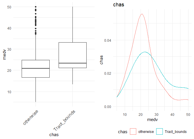
2. There seems to be significant difference between the houses that are Charles River track-bound or otherwise.

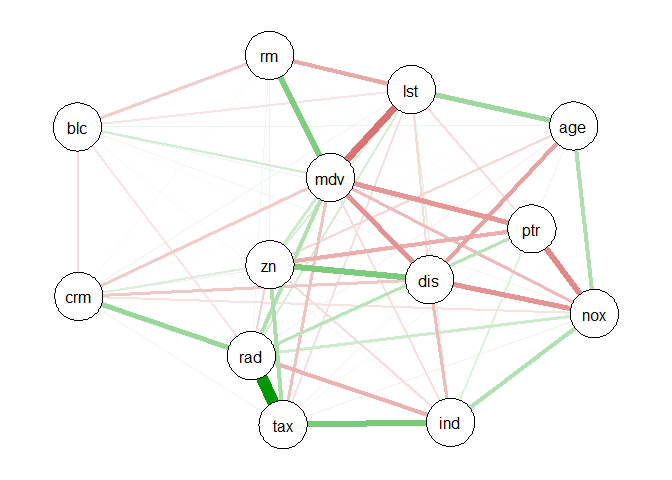
Correlation¶

The correlation between different variables is as follows

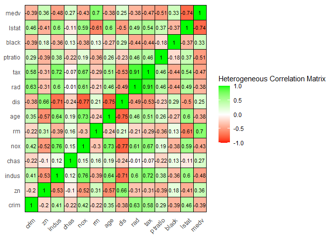
Observations:
1. There is a lot of correlation between many location based features like dis and nox, dist and indus, dist and age, rm and lstat, lstat and indus etc. The correlations between different (continuous) variables can be visualized below.

Initial Model Training¶

For my initial model, I am training using step wise linear regression. In every step, I want to observe the following:
1. What variables are added or removed from the model. The current model pics the column which gives the greatest decrease in AIC. The model stops when the decrease in AIC w.r.t. null(no change) is lower than the threshold.
2. Substantial increase/decrease in $\beta$ or change in its sign (which may be due to collinearity between the dependent variables)

## Start:  AIC=1297.43
## .outcome ~ crim + zn + indus + chasTract_bounds + nox + rm + 
##     age + dis + tax + ptratio + black + lstat + rad_catloc24
## 
##                    Df Sum of Sq     RSS    AIC
## - age               1      0.72  9208.4 1295.5
## - indus             1      3.76  9211.5 1295.6
## <none>                           9207.7 1297.4
## - chasTract_bounds  1     97.13  9304.8 1299.7
## - tax               1    118.38  9326.1 1300.6
## - zn                1    168.98  9376.7 1302.8
## - black             1    191.17  9398.9 1303.8
## - crim              1    307.05  9514.7 1308.8
## - rad_catloc24      1    314.92  9522.6 1309.1
## - nox               1    352.63  9560.3 1310.7
## - ptratio           1    957.94 10165.6 1335.7
## - dis               1    994.35 10202.0 1337.2
## - rm                1   1892.99 11100.7 1371.5
## - lstat             1   2127.87 11335.6 1380.0
## 
## Step:  AIC=1295.46
## .outcome ~ crim + zn + indus + chasTract_bounds + nox + rm + 
##     dis + tax + ptratio + black + lstat + rad_catloc24
## 
##                    Df Sum of Sq     RSS    AIC
## - indus             1      3.65  9212.1 1293.6
## <none>                           9208.4 1295.5
## + age               1      0.72  9207.7 1297.4
## - chasTract_bounds  1     97.93  9306.3 1297.8
## - tax               1    118.46  9326.9 1298.7
## - zn                1    168.59  9377.0 1300.8
## - black             1    193.24  9401.6 1301.9
## - crim              1    306.48  9514.9 1306.8
## - rad_catloc24      1    314.22  9522.6 1307.1
## - nox               1    369.87  9578.3 1309.5
## - ptratio           1    960.19 10168.6 1333.8
## - dis               1   1087.43 10295.8 1338.9
## - rm                1   1970.22 11178.6 1372.4
## - lstat             1   2321.66 11530.1 1385.0
## 
## Step:  AIC=1293.62
## .outcome ~ crim + zn + chasTract_bounds + nox + rm + dis + tax + 
##     ptratio + black + lstat + rad_catloc24
## 
##                    Df Sum of Sq     RSS    AIC
## <none>                           9212.1 1293.6
## + indus             1      3.65  9208.4 1295.5
## + age               1      0.61  9211.5 1295.6
## - chasTract_bounds  1     95.50  9307.6 1295.8
## - tax               1    152.24  9364.3 1298.3
## - zn                1    174.02  9386.1 1299.2
## - black             1    196.27  9408.3 1300.2
## - crim              1    303.79  9515.9 1304.8
## - rad_catloc24      1    335.42  9547.5 1306.2
## - nox               1    417.91  9630.0 1309.7
## - ptratio           1    982.91 10195.0 1332.9
## - dis               1   1125.61 10337.7 1338.5
## - rm                1   2045.55 11257.6 1373.2
## - lstat             1   2330.94 11543.0 1383.4

## 
## Call:
## lm(formula = .outcome ~ crim + zn + chasTract_bounds + nox + 
##     rm + dis + tax + ptratio + black + lstat + rad_catloc24, 
##     data = dat)
## 
## Residuals:
##      Min       1Q   Median       3Q      Max 
## -16.1877  -2.7794  -0.5639   1.8186  26.2200 
## 
## Coefficients:
##                    Estimate Std. Error t value Pr(>|t|)    
## (Intercept)       35.638467   5.799094   6.146 1.95e-09 ***
## crim              -0.125142   0.034673  -3.609 0.000347 ***
## zn                 0.042184   0.015443   2.732 0.006585 ** 
## chasTract_bounds   2.030470   1.003385   2.024 0.043682 *  
## nox              -17.255174   4.076237  -4.233 2.87e-05 ***
## rm                 4.120294   0.439949   9.365  < 2e-16 ***
## dis               -1.476732   0.212563  -6.947 1.54e-11 ***
## tax               -0.010071   0.003942  -2.555 0.010994 *  
## ptratio           -0.961287   0.148073  -6.492 2.55e-10 ***
## black              0.008800   0.003033   2.901 0.003928 ** 
## lstat             -0.526372   0.052651  -9.997  < 2e-16 ***
## rad_catloc24       5.669076   1.494858   3.792 0.000173 ***
## ---
## Signif. codes:  0 '***' 0.001 '**' 0.01 '*' 0.05 '.' 0.1 ' ' 1
## 
## Residual standard error: 4.829 on 395 degrees of freedom
## Multiple R-squared:  0.7474, Adjusted R-squared:  0.7404 
## F-statistic: 106.2 on 11 and 395 DF,  p-value: < 2.2e-16

Summary:
1. Initially all the factors were considered in the model.
2. By removing age from the initial model, the AIC is 1295.5 vs 1297.43 in the initial model. Therefore, age was removed.
3. By removing industry from the initial model, the AIC is 1293.6 vs the AIC of 1297.43. Therefore, industry was removed.
4. Adding or removing any other variable does not decrease AIC significantly. The remaining factors are the best factors of the final model.

Observations:
1. For every unit increase in crime, the price decreases by 0.12 units.
2. For every large residential properties, the price increases by 0.0421 units.
3. For every unit increase in NOX(pollution) levels, the price decreases by -17.25 units.
4. The presence of Charles River in track bounds increases the price of the property by 2.03 units.
5. One extra room increases the price by 4.12
6. Increase in average distance from work centres by 1 unit decreases the price by 1.47 units.
7. Increase in tax by one unit decreases the price by -0.01 units.
8. Surprisingly, increasing the parent teacher ratio by one unit, decreases the price by 0.96 units.
9. Racial discrimination is still an important factor.
10. One unit increase of lower status of the population decreases the price by 0.52 units.
11. The presence of 'rad=24' increases the price by 5.6 units.

Model diagnostics¶

I want to look at R-Squared and adjusted R-Square of the model on the test data. R-Square explains the proportion of variation in $y$ explained by our dependent variables. Then I want to look at the statistical significance of individual variables (using t-test) and validation of complete model (using F test). Some basic assumptions for doing the tests are validated using residual analysis, and finally I will look into multi-collinearity.

The R-Squared and RMSE of the model on test data are:¶

##      RMSE  Rsquared       MAE 
## 4.5506048 0.6797879 3.2017260

R-Square remains similar on the test set. Therefore, we are not over-fitting.

Testing statistical significance of individual dependent variables¶

The Null hypothesis and alternate hypothesis for each of the dependent variables $i$ is: $$ H_0 : \beta_i= 0 $$ $$ H_1 : \beta_i \neq 0 $$ The statistical significance can be validated using a t-test.

Validating the complete model¶

The null and alternate hypothesis for the model $y = \beta_0 + \beta_1x_1 + \beta_2x_2+...+\beta_kx_k + \epsilon$ is: $$ H_0 : \beta_1 = \beta_2 = ... = \beta_k = 0 $$ $$ H_1 : Not \, all\, \beta_i \,are\, 0 $$ The statistical significance can be validated using F test.

## 
## Call:
## lm(formula = .outcome ~ crim + zn + chasTract_bounds + nox + 
##     rm + dis + tax + ptratio + black + lstat + rad_catloc24, 
##     data = dat)
## 
## Residuals:
##      Min       1Q   Median       3Q      Max 
## -16.1877  -2.7794  -0.5639   1.8186  26.2200 
## 
## Coefficients:
##                    Estimate Std. Error t value Pr(>|t|)    
## (Intercept)       35.638467   5.799094   6.146 1.95e-09 ***
## crim              -0.125142   0.034673  -3.609 0.000347 ***
## zn                 0.042184   0.015443   2.732 0.006585 ** 
## chasTract_bounds   2.030470   1.003385   2.024 0.043682 *  
## nox              -17.255174   4.076237  -4.233 2.87e-05 ***
## rm                 4.120294   0.439949   9.365  < 2e-16 ***
## dis               -1.476732   0.212563  -6.947 1.54e-11 ***
## tax               -0.010071   0.003942  -2.555 0.010994 *  
## ptratio           -0.961287   0.148073  -6.492 2.55e-10 ***
## black              0.008800   0.003033   2.901 0.003928 ** 
## lstat             -0.526372   0.052651  -9.997  < 2e-16 ***
## rad_catloc24       5.669076   1.494858   3.792 0.000173 ***
## ---
## Signif. codes:  0 '***' 0.001 '**' 0.01 '*' 0.05 '.' 0.1 ' ' 1
## 
## Residual standard error: 4.829 on 395 degrees of freedom
## Multiple R-squared:  0.7474, Adjusted R-squared:  0.7404 
## F-statistic: 106.2 on 11 and 395 DF,  p-value: < 2.2e-16

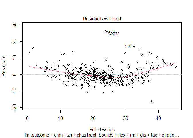
From the above summary, I can observe that the Pr(>|t|) or p-value is less than the cut-off value of $\alpha = 0.05$ for all variables. Also, the F-Statistic is 106.2 with a p value <2.2e-16. Thus, I reject both the above null hypothesis. The model is statistically significant.

Residual analysis¶

Some assumptions in the above hypothesis tests are:
1. The mean of errors should be zero
2. The variance of the errors should be constant across $y$
3. The errors should be random. They should follow a random distribution

I can validate these three assumptions using the residual plots

## 
## Call:
## lm(formula = .outcome ~ crim + zn + chasTract_bounds + nox + 
##     rm + dis + tax + ptratio + black + lstat + rad_catloc24, 
##     data = dat)
## 
## Coefficients:
##      (Intercept)              crim                zn  chasTract_bounds  
##         35.63847          -0.12514           0.04218           2.03047  
##              nox                rm               dis               tax  
##        -17.25517           4.12029          -1.47673          -0.01007  
##          ptratio             black             lstat      rad_catloc24  
##         -0.96129           0.00880          -0.52637           5.66908  
## 
## 
## ASSESSMENT OF THE LINEAR MODEL ASSUMPTIONS
## USING THE GLOBAL TEST ON 4 DEGREES-OF-FREEDOM:
## Level of Significance =  0.05 
## 
## Call:
##  gvlma(x = model$finalModel) 
## 
##                     Value   p-value                   Decision
## Global Stat        650.35 0.000e+00 Assumptions NOT satisfied!
## Skewness           125.66 0.000e+00 Assumptions NOT satisfied!
## Kurtosis           385.33 0.000e+00 Assumptions NOT satisfied!
## Link Function      120.98 0.000e+00 Assumptions NOT satisfied!
## Heteroscedasticity  18.39 1.803e-05 Assumptions NOT satisfied!

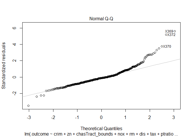
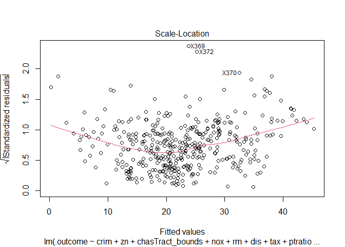
Observations:
None of the three conditions are properly satisfied. Certain outlier points seem to have a huge effect on the residuals and the model. As normality conditions are not met, I cannot trust the p values from above t and F statistics.

Multi-collinearity¶

From the correlation matrix, I am expecting large multicollinearity between the features.

Variation inflation factor is the value by which the square of the estimate is inflated in presence of multi-collinearity. The t-statistic is thus deflated by $\sqrt(VIF)$ and standard error of estimate is inflated by $\sqrt(VIF)$.
$$ VIF = \frac{1}{1-(R_j)^2} $$ Where $R_j$ is the regression correlation coefficient between $j$th variable and all other dependent variables.
A VIF of greater than 10 is considered bad. (decreases the t-value ~3.16 times, thus increasing p-value)

##             crim               zn chasTract_bounds              nox 
##         1.733555         2.394835         1.050701         3.810818 
##               rm              dis              tax          ptratio 
##         1.825246         3.581245         7.671215         1.855131 
##            black            lstat     rad_catloc24 
##         1.320648         2.551655         7.602218

The t-value for tax and rad_cat variables are inflated by $\sqrt(VIF) = \sqrt(7.6) =2.7$. The corrected t-value would be
$$ t_{actual} = \frac{\beta_i}{S_e(\beta_i)} * \sqrt(VIF) = t_{pred}\sqrt(VIF$$ Where t-predicted is the value of t in the summary table. Increasing t-value by ~2.7% decreases p further, and as both the values *tax and rad_cat have p-values below 5%, increasing the t-value further will only decrease the p-value further making the two variables more significant.

Testing over-fitting¶

To prevent over fitting, it is important to find the ideal number of independent variables. Mallows's $C_p$ is used to identify the ideal number of features in the model. The best regression model is the model with the number of parameters close to $C_p$.

$$ C_p = \frac{SSE_p}{MSE_{full}} -(N-2p) $$ Where N is the number of observations and p is the number of parameters.
The Mallows cp in our case is:

## [1] 10.18672

The number of features that are significant in the current model is 11.

Auto correlation¶

Durbin watson is a hypothesis test to test the existence of auto correlation. The null and alternate hypothesis are:
$$ H_0 : \rho_i= 0 $$ $$ H_1 : \rho_i \neq 0 $$ The test statistic is the Durbin Watson statistic $D$. D is between 0 and 4. D close to 2 implies absence of auto correlation.

##  lag Autocorrelation D-W Statistic p-value
##    1       0.4198705      1.144239       0
##  Alternative hypothesis: rho != 0

As p value is less than cut-off at $\alpha =0.05$, there is no auto correlation. Auto correlation generally exists in time series data.

Outlier analysis¶

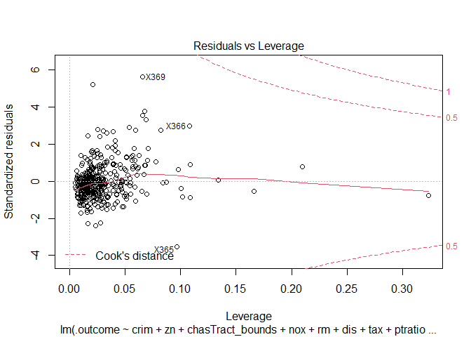
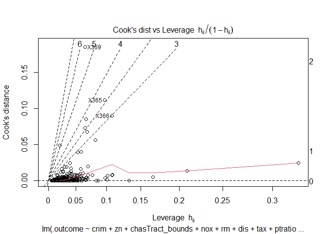
From the residual plots, I suspect that that there might be certain outliers that are adversely effecting the model. I am using the following distance measures to check for outliers in the model.
1. Mahalanobis distance: Distance between the observation and the centroid of the values
2. Leverages: Capacity of an observation to be influential due to having extreme predictor values (unusual combination of predictor values).
3. Jackknife residuals (studentized residual): Division of residuals by its standard deviation
4. Cook's distance': Detects observations that have a disproportionate impact on the determination of the model parameters (large change in parameters if deleted).
5. DFBETAS: Changes in coefficients when the observations are deleted.
6. DFFITS: Change in the fitted value when the observation is deleted (standardized by the standard error)
7. hat: Diagonal elements of the hat matrix
8. cov.r: Co-variance ratios

The above metrics for sample 5 observations, and outlier plots (for significant metrics) are as follows:

Outlier metrics
	dfb.1_	dfb.crim	dfb.zn	dfb.chT_	dfb.nox	dfb.rm	dfb.dis	dfb.tax	dfb.ptrt	dfb.blck	dfb.lstt	dfb.r_24	dffit	cov.r	cook.d	hat	maha
X369	0.7796401	-0.2317501	0.1678140	-0.0579735	-0.0936772	-1.1097413	-0.4805830	-0.0144256	-0.0745656	0.0747545	-1.1868934	0.4152958	1.5508236	0.4063263	0.1848802	0.0656965	59.32389
X419	0.0147891	0.3645414	-0.0178977	0.0107611	0.0119382	-0.0058155	0.0304393	0.0005552	0.0161723	-0.1159999	-0.0610864	-0.0882379	0.4029018	1.2799527	0.0135408	0.2094680	80.63853
X411	0.0050986	0.0114598	-0.0002544	0.0003139	-0.0021656	-0.0040736	-0.0019297	0.0004132	0.0001400	-0.0077489	-0.0068897	-0.0021726	0.0159856	1.1901705	0.0000213	0.1338773	55.40362
X406	0.0201748	-0.2245737	0.0051880	-0.0027568	-0.0129879	-0.0007893	-0.0145494	-0.0025818	-0.0039595	-0.0563659	0.0126108	0.0401276	-0.2356062	1.2262623	0.0046343	0.1664139	65.24982
X381	0.0980385	-0.5245638	0.0341992	-0.0047776	-0.0327019	-0.0832358	-0.0461418	-0.0290283	-0.0292670	-0.1138749	0.0386572	0.1235709	-0.5425691	1.4946534	0.0245556	0.3231086	126.23671

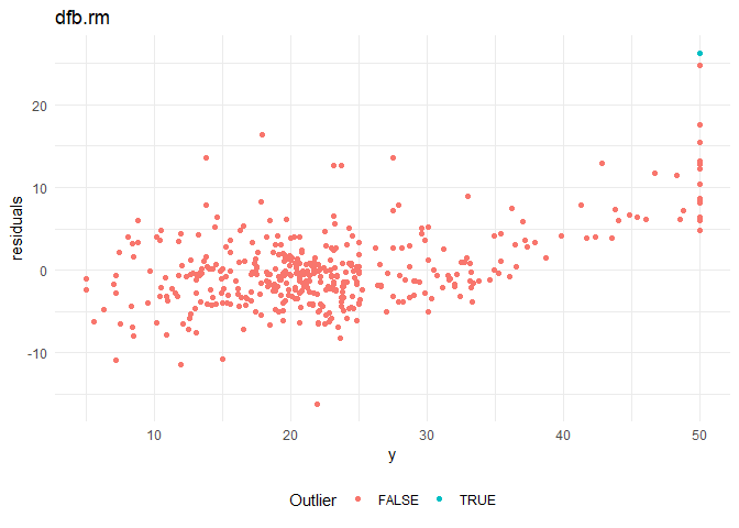
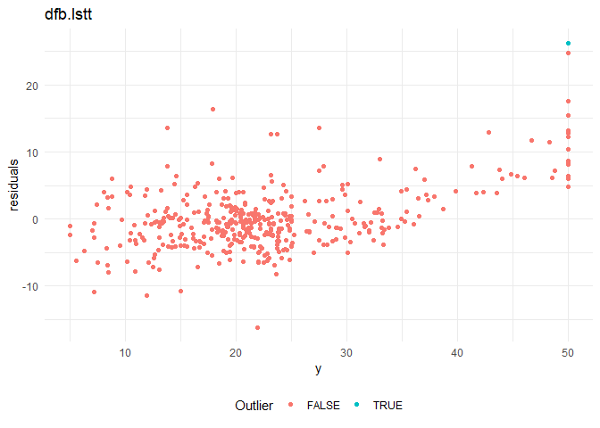
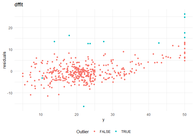
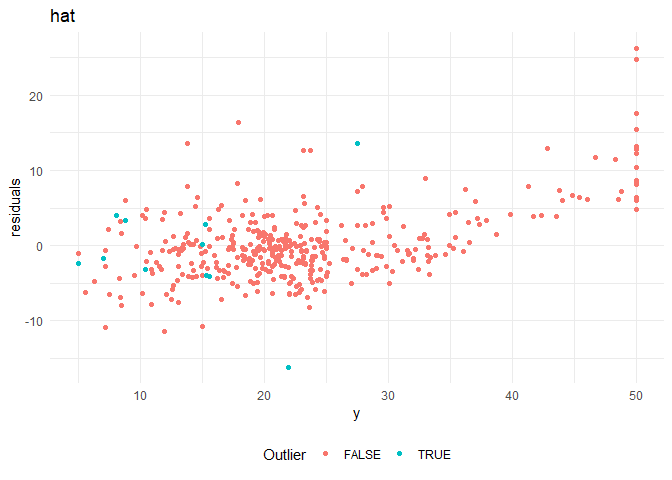
Cooks distance and leverage values plots: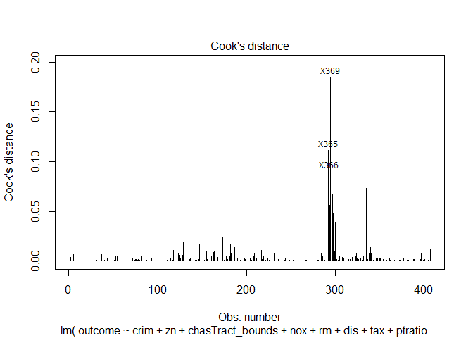

Building a better model¶

Now that I know all the problems that are present in the current model, I build a better model taking care of all of them. The current model has the following problems:
1. Residuals are not normally distributed
2. Residuals do not have constant variance
3. Multicollinearity among variables
4. Outliers affecting $\beta$ coefficients
5. Low R-Squared

A slightly better model than the above is shown below.

## 
## Call:
## lm(formula = .outcome ~ rm + `I(1/rm)` + `poly(dis, degree = 2)2` + 
##     `I(1/dis)` + `I(1/ptratio)` + `exp(black)` + `log(lstat)` + 
##     `sqrt(lstat)` + `poly(crim, degree = 2)1` + `poly(crim, degree = 2)2` + 
##     `exp(indus)` + nox + `I(1/tax)` + rad_catloc24 + `rm:lstat`, 
##     data = dat)
## 
## Residuals:
##      Min       1Q   Median       3Q      Max 
## -21.8040  -2.1502  -0.0956   1.9586  21.2613 
## 
## Coefficients:
##                              Estimate  Std. Error t value Pr(>|t|)    
## (Intercept)                -8.295e+01   1.535e+01  -5.404 1.14e-07 ***
## rm                          1.107e+01   1.260e+00   8.786  < 2e-16 ***
## `I(1/rm)`                   1.990e+02   5.071e+01   3.925 0.000102 ***
## `poly(dis, degree = 2)2`   -9.122e+00   4.170e+00  -2.188 0.029294 *  
## `I(1/dis)`                  1.965e+01   2.167e+00   9.070  < 2e-16 ***
## `I(1/ptratio)`              1.815e+02   3.119e+01   5.821 1.22e-08 ***
## `exp(black)`              -6.794e-173   0.000e+00    -Inf  < 2e-16 ***
## `log(lstat)`               -2.062e+01   2.729e+00  -7.554 3.02e-13 ***
## `sqrt(lstat)`               1.792e+01   3.439e+00   5.211 3.04e-07 ***
## `poly(crim, degree = 2)1`  -5.309e+01   6.468e+00  -8.208 3.29e-15 ***
## `poly(crim, degree = 2)2`   2.435e+01   5.810e+00   4.191 3.44e-05 ***
## `exp(indus)`               -5.070e-12   2.015e-12  -2.516 0.012264 *  
## nox                        -2.090e+01   3.323e+00  -6.290 8.48e-10 ***
## `I(1/tax)`                  1.248e+03   2.990e+02   4.173 3.70e-05 ***
## rad_catloc24                5.340e+00   9.906e-01   5.391 1.22e-07 ***
## `rm:lstat`                 -2.391e-01   5.106e-02  -4.684 3.89e-06 ***
## ---
## Signif. codes:  0 '***' 0.001 '**' 0.01 '*' 0.05 '.' 0.1 ' ' 1
## 
## Residual standard error: 3.664 on 391 degrees of freedom
## Multiple R-squared:  0.8561, Adjusted R-squared:  0.8506 
## F-statistic:   155 on 15 and 391 DF,  p-value: < 2.2e-16

Modelling is an iterative process. With more effort, I could get a better model using linear regression itself. Otherwise, I could use other regression techniques to get better results.