Linear Programming (R)
Simple minimization problem
This Problem is taken from An Introduction to Management Science : Quantitative Approach to Decision Making book. It is the example problem at page 52, chapter 2,5.
In this blog I will try to understand how to solve simple linear programming problems using R.
Problem
M&D Chemicals produces two products that are sold as raw materials to companies manufacturing bath soaps and laundry detergents. Based on an analysis of current inventory levels and potential demand for the coming month, M&D's management specified that the combined production for products A and B must total at least 350 gallons. Separately, a major customer's order for 125 gallons of product A must also be satisfied. Product 'A' requires 2 hours of processing time per gallon and product B requires 1 hour of processing time per gallon. For the coming month, 600 hours of processing time are available. M&D's objective is to satisfy these requirements at a minimum total production cost. Production costs are 2 dollars per gallon for product A and 3 dollars per gallon for product B.
Suppose additionally there is a constraint that the maximum production for B is 400 gallons.
Solution
The decision variables and objective function for the problem is as follows:
\(x_A\) = number of gallons of product A
\(x_B\) = number of gallons of product B
With production costs at 2 dollars per gallon for product A and 3 dollars per gallon for product B, the objective function that corresponds to the minimization of the total production cost can be written as
$$ Min( 2x_A + 3x_B) $$ The different constraints for the problem will be as follows:
1. To satisfy the major customer's demand for 125 gallons of product A, we know A must be at least 125.
$$ x_A \geq 125 $$ 2. The combined production for both products must total at least 350 gallons
$$ x_A + x_B \geq 350 $$ 3. The available processing time must not exceed 600 hours
$$ 2x_A+x_B \leq 600 $$ 4. The production of B cannot exceed 400 gallons
$$ x_b \leq 400 $$ 5. As the production of A or B cannot be negative.
$$ x_A \geq 0, x_B \geq 0 $$
Formulation
Combining all the constraints, the LP can be written as:
$$ Min(2x_A + 3x_B) $$ Subject to constraints:
| A | B | RHS | |
|---|---|---|---|
| 1 | 0 | \(\geq\) | 125 |
| 1 | 1 | \(\geq\) | 350 |
| 2 | 1 | \(\leq\) | 600 |
| 0 | 1 | \(\leq\) | 400 |
Graphical solution
Plotting the constraints I get the shaded region as the intersection region which satisfies all the constraints. Solutions that satisfy all the constraints are termed feasible solutions, and the shaded region is called the feasible solution region, or simply the feasible region.
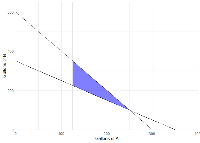
From the above plot, I observe that \(x_b < 400\) is a redundant constraint.
To find the minimum-cost solution, we now draw the objective function line corresponding to a particular total cost value. For example, we might start by drawing the line \(2x_A + 3x_B = 1200\). This line is shown in below simulation.
Clearly, some points in the feasible region would provide a total cost of $1200. To find the values of A and B that provide smaller total cost values, we move the objective function line in a lower left direction until, if we moved it any farther, it would be entirely outside the feasible region. Note that the objective function line \(2x_A + 3x_B = 800\) intersects the feasible region at the extreme point \(x_A = 250\) and \(x_B = 100\). This extreme point provides the minimum-cost solution with an objective function value of 800.
Therefore the ideal production to minimize cost should be to produce 250 gallons of A and 100 gallons of B.
Solution in R
In R, LP_solve is implemented through the lpSolve and lpSolveAPI packages. Using the lpSolve package, I can solve a linear programming problem as follows:
library(lpSolve)

# A matrix of LHS of constraints (except the non negative)
constraints.LHS <- matrix(c(1,0,
              1,1,
              2,1,
              0,1), nrow = 4, byrow = TRUE)

# A list of RHS of constraints (except the non negative)
RHS <- c(125, 350, 600,400)

# A list of the constraints directions (except the non negative)
constranints_direction  <- c(">=", ">=", "<=", '<=')

# A list of objective function coefficients
objective.fxn <- c(2,3)

# Find the optimal solution
optimum <-  lp(direction="min",
               objective.in = objective.fxn,
               const.mat = constraints.LHS,
               const.dir = constranints_direction,
               const.rhs = RHS,
               all.int = T,
               compute.sens = TRUE)
The result of the above (after formatting) is:
## Success: the objective function is 800
| Variable | Optimum.Value | Reduced.Cost | Objective.coefficient | Allowable.decrease | Allowable.Increase |
|---|---|---|---|---|---|
| A | 250 | 0 | 2 | -1e+30 | 3 |
| B | 100 | 0 | 3 | 2 | 1e+30 |
| Constraint | Dual.Value | Slack.Surplus | RHS.Value | Allowable.Decrease.to | Allowable.Increase.to |
|---|---|---|---|---|---|
| 1 | 0 | 125 | 125 | -1e+30 | 1e+30 |
| 2 | 4 | 0 | 350 | 300 | 475 |
| 3 | -1 | 0 | 600 | 475 | 700 |
| 4 | 0 | -300 | 400 | -1e+30 | 1e+30 |
| 5 | 0 | 250 | 0 | -1e+30 | 1e+30 |
| 6 | 0 | 100 | 0 | -1e+30 | 1e+30 |
Sensitivity analysis
Sensitivity analysis is the study of how the changes in the coefficients of an optimization model affect the optimal solution. Using sensitivity analysis, we can answer questions such as the following:
1. How will a change in a coefficient of the objective function affect the optimal solution?
2. How will a change in the right-hand-side value for a constraint affect the optimal solution?
From the above solution, I observe the following
1. The current price coefficient of A is 2 and the current price coefficient of B is 3. The optimal solution will remain the same even if the price of A is 3 keeping the price of B constant, or if the price of B is 2 keeping A constant. This can be visualized above.
2. The binding constraints ie: processing time and production of both products have a Slack/Surplus values of zero. The other non binding constraints have positive/negative slack values. Slack values represent the unused capacity.
3. The dual value associated with a constraint is the change in the optimal value of the solution per unit increase in the right-hand side of the constraint. For example, if I increased the minimum production constraint from 350 to 351, The cost of production will increase by 4 dollars. Similarly if I could increase the available processing time to 601 hours instead of 600 hours, the cost will decrease by 1 dollar. The range in which this increase or decrease is applicable is also given. This can be visualized in the above simulation.