Exploratory factor analysis (R)
Factor analysis
Factor analysis can be performed to combine a large number of variables to smaller number of factors. This is done usually for the following reasons:
1. Find interrelationships among different kinds of variables
2. Identify common underlying dimension
3. Data reduction and removing duplicate columns
Among the many types of ways one can do factor analysis, two ways are popular. They are
1. Principal component analysis
2. Common factor analysis
PCA considers the total variance in the data while CFA only considers the common variance. In this blog, we are going to discuss Principal component analysis.
Principal component analysis
PCA is the most widely used exploratory factor analysis technique, It is developed by Pearson and Hotelling. The objective of PCA is to rigidly rotate the axes of p-dimensional space to new positions (principal axes) that have the following properties:
1. Ordered such that principal axis 1 has the highest variance, axis 2 has the next highest variance, ...., and axis p has the lowest variance
2. Covariance among each pair of the principal axes is zero (the principal axes are uncorrelated)
Data and problem
This dataset contains 90 responses for 14 different variables that customers consider while purchasing car. The survey questions were framed using 5-point likert scale with 1 being very low and 5 being very high. The data can be downloaded from this link. The variables were the following:
1. Price
2. Safety
3. Exterior looks
4. Space and comfort
5. Technology
6. After sales service
7. Resale value
8. Fuel type
9. Fuel efficiency
10. Colour
11. Maintenance
12. Test drive
13. Product reviews
14. Testimonials
A sample of the data is shown:
| Price | Safety | Exterior_Looks | Space_comfort | Technology | After_Sales_Service | Resale_Value | Fuel_Type | Fuel_Efficiency | Color | Maintenance | Test_drive | Product_reviews | Testimonials |
|---|---|---|---|---|---|---|---|---|---|---|---|---|---|
| 4 | 4 | 5 | 5 | 5 | 5 | 5 | 4 | 3 | 3 | 4 | 4 | 3 | 4 |
| 4 | 4 | 4 | 5 | 5 | 5 | 1 | 5 | 3 | 3 | 3 | 4 | 4 | 5 |
| 3 | 4 | 3 | 4 | 4 | 4 | 2 | 3 | 4 | 3 | 3 | 3 | 4 | 4 |
| 4 | 4 | 5 | 4 | 3 | 4 | 5 | 4 | 4 | 2 | 4 | 2 | 4 | 3 |
| 4 | 4 | 4 | 5 | 5 | 5 | 2 | 4 | 4 | 4 | 4 | 4 | 4 | 5 |
KMO Index
The Kaiser-Meyer-Olkin (KMO) measure of sampling adequacy is an index used to examine the appropriateness of factor analysis. High values (between 0.5 and 1.0) indicate factor analysis is appropriate. Values below 0.5 imply that factor analysis may not be appropriate
## Kaiser-Meyer-Olkin factor adequacy
## Call: KMO(r = efa)
## Overall MSA =  0.61
## MSA for each item =
##               Price              Safety      Exterior_Looks       Space_comfort
##                0.72                0.47                0.55                0.61
##          Technology After_Sales_Service        Resale_Value           Fuel_Type
##                0.65                0.62                0.63                0.68
##     Fuel_Efficiency               Color         Maintenance          Test_drive
##                0.62                0.56                0.61                0.64
##     Product_reviews        Testimonials
##                0.69                0.50
Bartlett's test of sphericity
Bartlett's test of sphericity is a test statistic used to examine the hypothesis that the variables are uncorrelated in the population. In other words, the population correlation matrix is an identity matrix; each variable correlates perfectly with itself (r = 1) but has no correlation with the other variables (r = 0).
\(H_0\): All non-diagonal values of correlation matrix are zero
\(H_1\): Not all diagonal values of correlation matrix are zero
##
##  Bartlett's test of sphericity
##
## data:  efa
## X-squared = 247.71, df = 91, p-value < 2.2e-16
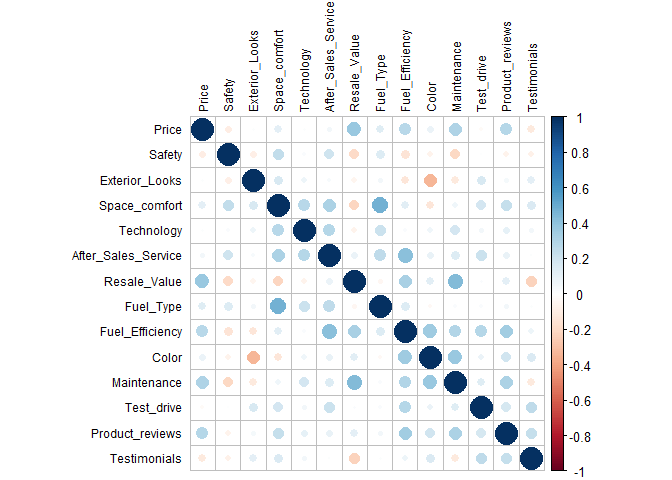
From the above correlation matrix and the test we can observe that there is some dependence between the variables and factor analysis can therefore be performed.
In this example, the factors can be considered as the underlying thought process while each variable can be considered as the response to the question. While looking for comfort in a car, a person might look into aesthetics, functionality, economic value and credibility. These are factors while the survey questions are variables.
While replying to a question in a survey, for every variable, the respondent underlying thought process gives weightage to each factor as a function of that variable. This can be written as (for normalized variables):
$$ y_1 = \lambda_{11} f_1 + \lambda_{12} f_2 + \cdots + \lambda_{1m} f_m + \epsilon_1 $$ $$ y_2 = \lambda_{21} f_1 + \lambda_{22} f_2 + \cdots + \lambda_{2m} f_m + \epsilon_2 $$ $$ ... $$ $$ y_p = \lambda_{p1} f_1 + \lambda_{p2} f_2 + \cdots + \lambda_{pm} f_m + \epsilon_p $$ Where \(f_1, f_2 \cdots\) are the factors and \(y_1, y_2 \cdots\) are variables. \(\lambda_{pm}\) are called factor loadings, or the correlation between variables and factors.
Number of factors
The number of factors to decompose the dataset should be selected. There are multiple ways of doing it, the most popular ones are:
1. Number of eigenvalues greater than 1
2. Scree plot
3, Percentage of variation explained
Let us look at each one of them:
Eigen values
The eigenvalue represents the total variance explained by each factor. If each variable is normalized before the analysis, the maximum eigen value of all the factors combined should be equal to the number of variables (As normalized variables have variation as 1)
The eigen values(from the co-variance matrix) for this data set is:
##  [1] 2.1585694 1.6836760 1.0709449 0.9760982 0.7723481 0.6364842 0.5211956
##  [8] 0.4245587 0.3942269 0.3600300 0.2747809 0.2306904 0.1774646 0.1588822
Any factor which has eigen value less than 1 explains the variation less than the variation explained by a variable. So one way to identify the number of factors is the number of eigenvalues greater than 1. From the eigen values, the number of factors to consider is 3.
Scree plot
A scree plot is a line plot of the eigenvalues of factors or principal components in an analysis. A scree plot always displays the eigenvalues in a downward curve, ordering the eigenvalues from largest to smallest. According to the scree test, the "elbow" of the graph where the eigenvalues seem to level off is found and factors or components to the left of this point should be retained as significant. It is named after its resemblance to scree(broken rock fragments at the base of cliffs) after its elbow.
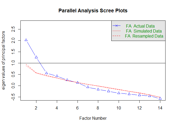
## Parallel analysis suggests that the number of factors = 4 and the number of components = NA
From the scree plot, a significant slope change can be observed after the third or fourth factor. The number of factors to consider from scree plot is 3.
After identifying the number of factors, the next step in PCA is to create the factors without rotation. This is done in such a way to satisfy:
1. Principal axis-1 has the highest variance, axis-2 has the next highest variance, .... , and axis p has the lowest variance
2. Co-variance among each pair of the principal axes is zero (the principal axes are uncorrelated)
##
## Call:
## factanal(x = ~., factors = 3, data = efa, na.action = na.exclude,     rotation = "none", cutoff = 0.3)
##
## Uniquenesses:
##               Price              Safety      Exterior_Looks       Space_comfort
##               0.721               0.896               0.849               0.277
##          Technology After_Sales_Service        Resale_Value           Fuel_Type
##               0.870               0.758               0.306               0.713
##     Fuel_Efficiency               Color         Maintenance          Test_drive
##               0.592               0.258               0.567               0.904
##     Product_reviews        Testimonials
##               0.782               0.854
##
## Loadings:
##                     Factor1 Factor2 Factor3
## Price                0.353   0.199   0.339
## Safety              -0.233   0.200
## Exterior_Looks      -0.281   0.127   0.238
## Space_comfort       -0.235   0.815
## Technology                   0.358
## After_Sales_Service  0.149   0.466
## Resale_Value         0.618  -0.116   0.547
## Fuel_Type                    0.524
## Fuel_Efficiency      0.538   0.341
## Color                0.678          -0.526
## Maintenance          0.608   0.208   0.141
## Test_drive           0.112   0.286
## Product_reviews      0.296   0.361
## Testimonials                 0.208  -0.318
##
##                Factor1 Factor2 Factor3
## SS loadings      1.945   1.813   0.897
## Proportion Var   0.139   0.130   0.064
## Cumulative Var   0.139   0.268   0.333
##
## Test of the hypothesis that 3 factors are sufficient.
## The chi square statistic is 65.94 on 52 degrees of freedom.
## The p-value is 0.0925
The sum of square loading (SS Loadings) represents the eigen values of each loading.
The uniqueness of each variable is also shown. \(Uniqueness=1−Communality\) where Communality is the SS of all the factor loadings for a given variable. If all the factors jointly explain a large percent of variance in a given variable, that variable has high Communality (and thus low uniqueness).
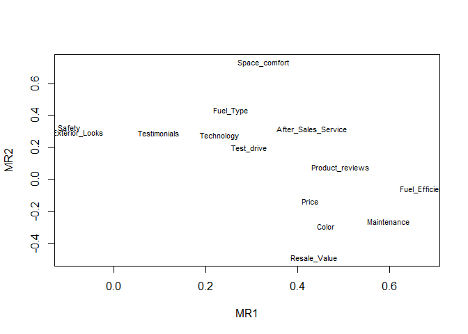
Our goal is to name the factors. Sometimes visualizations help. Plotting the factor loadings for the first two factors.
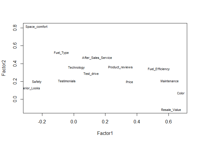
It can be difficult to label factors when they are unrotated, since a description of one factor might overlap with a description of another factor. We can rotate the factors to obtain more straightforward interpretations. Rotations are of various types:
1. Varimax rotation: An orthogonal rotation method that minimizes the number of variables that have high loadings on each factor. This method simplifies the interpretation of the factors
2. Quartimax rotation: A rotation method that minimizes the number of factors needed to explain each variable. This method simplifies the interpretation of the observed variables
3. Equamax rotation: A rotation method that is a combination of the varimax method, which simplifies the factors, and the quartimax method which simplifies the variables
4. Direct Oblimin Method: A method for oblique (non-orthogonal) rotation
5. Promax rotation: An oblique rotation, which allows factors to be correlated
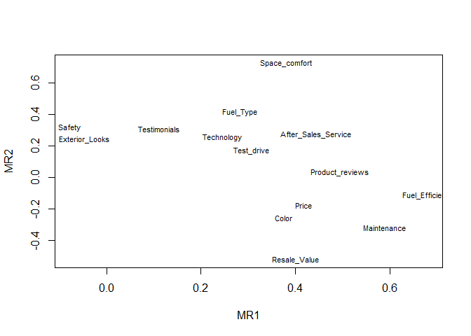
The loadings for oblimin method is shown:
##
## Loadings:
##                     MR1    MR2    MR3
## Fuel_Efficiency      0.682
## Maintenance          0.591 -0.315
## Product_reviews      0.496
## After_Sales_Service  0.444
## Price                0.417
## Color                0.377
## Test_drive           0.308
## Space_comfort        0.381  0.725
## Resale_Value         0.402 -0.520
## Fuel_Type                   0.413
## Safety                      0.317
## Technology
## Exterior_Looks
## Testimonials                0.306  0.664
##
##                  MR1   MR2   MR3
## SS loadings    2.136 1.595 0.873
## Proportion Var 0.153 0.114 0.062
## Cumulative Var 0.153 0.267 0.329
##
## Loadings:
##                     MR1    MR2    MR3    MR4
## Fuel_Efficiency      0.679
## Maintenance          0.599
## Product_reviews      0.495
## Color                0.462         0.427 -0.356
## After_Sales_Service  0.432
## Price                0.428
## Test_drive
## Space_comfort               0.731
## Resale_Value         0.437 -0.495
## Fuel_Type                   0.430
## Technology
## Testimonials                       0.603
## Exterior_Looks                            0.485
## Safety
##
##                  MR1   MR2   MR3   MR4
## SS loadings    2.175 1.630 0.912 0.711
## Proportion Var 0.155 0.116 0.065 0.051
## Cumulative Var 0.155 0.272 0.337 0.388
Validation
The factors created can be validated by looking at error metrics, or TLI.
## Factor Analysis using method =  minres
## Call: fa(r = efa, nfactors = 4, rotate = "oblimin", fm = "minres")
## Standardized loadings (pattern matrix) based upon correlation matrix
##                       MR1   MR2   MR3   MR4   h2   u2 com
## Price                0.43 -0.14 -0.27  0.16 0.30 0.70 2.3
## Safety              -0.10  0.32 -0.11 -0.33 0.23 0.77 2.4
## Exterior_Looks      -0.08  0.29 -0.10  0.48 0.34 0.66 1.8
## Space_comfort        0.33  0.73 -0.15 -0.01 0.67 0.33 1.5
## Technology           0.23  0.27 -0.04 -0.08 0.13 0.87 2.2
## After_Sales_Service  0.43  0.31 -0.10 -0.19 0.33 0.67 2.4
## Resale_Value         0.44 -0.49 -0.32  0.16 0.57 0.43 3.0
## Fuel_Type            0.25  0.43 -0.22 -0.13 0.32 0.68 2.4
## Fuel_Efficiency      0.68 -0.06  0.08 -0.03 0.47 0.53 1.0
## Color                0.46 -0.29  0.43 -0.36 0.61 0.39 3.6
## Maintenance          0.60 -0.26 -0.08  0.02 0.44 0.56 1.4
## Test_drive           0.30  0.19  0.21  0.17 0.20 0.80 3.3
## Product_reviews      0.49  0.07  0.16  0.21 0.32 0.68 1.6
## Testimonials         0.10  0.29  0.60  0.23 0.51 0.49 1.8
##
##                        MR1  MR2  MR3  MR4
## SS loadings           2.18 1.63 0.91 0.71
## Proportion Var        0.16 0.12 0.07 0.05
## Cumulative Var        0.16 0.27 0.34 0.39
## Proportion Explained  0.40 0.30 0.17 0.13
## Cumulative Proportion 0.40 0.70 0.87 1.00
##
## Mean item complexity =  2.2
## Test of the hypothesis that 4 factors are sufficient.
##
## The degrees of freedom for the null model are  91  and the objective function was  2.97 with Chi Square of  247.71
## The degrees of freedom for the model are 41  and the objective function was  0.57
##
## The root mean square of the residuals (RMSR) is  0.05
## The df corrected root mean square of the residuals is  0.07
##
## The harmonic number of observations is  90 with the empirical chi square  38.46  with prob <  0.58
## The total number of observations was  90  with Likelihood Chi Square =  46.2  with prob <  0.27
##
## Tucker Lewis Index of factoring reliability =  0.922
## RMSEA index =  0.036  and the 90 % confidence intervals are  0 0.085
## BIC =  -138.29
## Fit based upon off diagonal values = 0.94
## Measures of factor score adequacy
##                                                   MR1  MR2  MR3  MR4
## Correlation of (regression) scores with factors   0.9 0.88 0.81 0.74
## Multiple R square of scores with factors          0.8 0.78 0.65 0.55
## Minimum correlation of possible factor scores     0.6 0.56 0.30 0.10
The Tucker-Lewis Index (TLI) is 0.93 – an acceptable value considering it’s over 0.9.
The correlation between the newly created factors is small
Interpreting the Factors
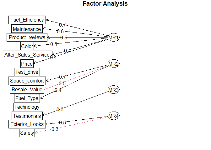
After establishing the adequacy of the factors, it’s time for us to interpret the factors. This is the theoretical side of the analysis where we form the factors depending on the variable loadings. In this case, here is how the factors can be created:
Factor 1 - Economic value:
Factor 1 contains resale value, maintenance, fuel efficiency and price. It is describing the Economic value of the car.
Factor 2 - Functional benefits:
Factor 2 contains Space_comfort, Fuel_Type, After_Sales_Service, Safety and Technology. It is describing the functional benefits of the car
Factor 3- Aesthetics
Factor 3 contains color and exterior looks. This factor is describing the Aesthetics of the car
Factor 4 - Credibility
Factor 4 contains Test drive, product reviews and testimonials. It is describing the credibility of the car
References
- Multivariate data analysis - Hair, Anderson, Black
- Factors affecting passenger satisfaction levels: a case study of Andhra Pradesh State Road Transport Corporation (India) - Nagadevara - trid.trb.org
- Promptcloud blog on EFA in R
- João Pedro Neto tutorials - Universidade de lisboa
- Penn state social science research institute tutorials
- Minato Nakazawa notes - Kobe University