Customer Lifetime Value

In this blog, I want to introduce Markov chains and find out the customer lifetime value. Customer Lifetime Value is the net present value (NPV) of the future margin generated from a customer or a customer segment.

Concept¶

Markov Chains¶

In probability theory and statistics, a sequence or other collection of random variables is independent and identically distributed (i.i.d) if each random variable has the same probability distribution as the others and all are mutually independent.
We have a set of states, S = {$s_1, s_2,...,s_r$}. The process starts in one of these states and moves successively from one state to another. Each move is called a step. If the chain is currently in state $s_i$, then it moves to state $s_j$ at the next step with a probability denoted by $p_{ij}$, and this probability does not depend upon which states the chain was in before the current state.

That is the probability to be present in state j at time t+1 is only dependent on the state at time t. $$ P_{ij} = P(X_{t+1} = j | X_{t} = i) $$

Customer Lifetime Value¶

Customer lifetime value is important because, the higher the number, the greater the profits. You'll always have to spend money to acquire new customers and to retain existing ones, but the former costs five times as much. When you know your customer lifetime value, you can improve it.

The customer segments can be represented as states of the Markov chain. Let {0, 1, 2, …, m} be the states of a Markov chain in which states {1, 2,..., m} denote different customer segments and state 0 denotes non-customer state.

The steady-state retention probability is given by $$ R_t = 1 - \frac{\pi_0(1-P_{00})}{1-\pi_0}$$ Where $P_{00}$ is the transition probability of State 0, and $\pi_0$ is the steady-state distribution for State 0.

Similarly, Customer lifetime value for N periods is given by:
$CLV = \sum_{t=0}^{N} \frac{P_I×P^t×R}{(1+i)^t}$
Where PI is the initial distribution of customers in different states, P is the transition probability matrix, R is the reward vector (margin generated in each customer segment). The interest rate is i (discount rate), $d = 1 + \frac{1}{1+i}$ is the discount factor.

Data¶

The data is obtained from the UCI machine learning repository. It is an Online Retail Data Set which contains all the transactions occurring between 01/12/2010 and 09/12/2011 for a UK-based and registered non-store online retail. The company mainly sells unique all-occasion gifts. Many customers of the company are wholesalers.

A sample data is shown below

raw_data
InvoiceNo	StockCode	Description	Quantity	InvoiceDate	UnitPrice	CustomerID	Country
579529	20750	RED RETROSPOT MINI CASES	2	2011-11-30 08:50:00	7.95	12488	France
568919	22615	PACK OF 12 CIRCUS PARADE TISSUES	12	2011-09-29 14:38:00	0.39	12937	United Kingdom
559521	22553	PLASTERS IN TIN SKULLS	7	2011-07-08 16:26:00	1.65	NA	Unspecified
569640	22961	JAM MAKING SET PRINTED	12	2011-10-05 12:25:00	1.45	12471	Germany
548542	22076	6 RIBBONS EMPIRE	12	2011-03-31 18:05:00	1.65	13918	United Kingdom

##   InvoiceNo          StockCode         Description           Quantity        
##  Length:541909      Length:541909      Length:541909      Min.   :-80995.00  
##  Class :character   Class :character   Class :character   1st Qu.:     1.00  
##  Mode  :character   Mode  :character   Mode  :character   Median :     3.00  
##                                                           Mean   :     9.55  
##                                                           3rd Qu.:    10.00  
##                                                           Max.   : 80995.00  
##                                                                              
##   InvoiceDate                    UnitPrice           CustomerID    
##  Min.   :2010-12-01 08:26:00   Min.   :-11062.06   Min.   :12346   
##  1st Qu.:2011-03-28 11:34:00   1st Qu.:     1.25   1st Qu.:13953   
##  Median :2011-07-19 17:17:00   Median :     2.08   Median :15152   
##  Mean   :2011-07-04 13:34:57   Mean   :     4.61   Mean   :15288   
##  3rd Qu.:2011-10-19 11:27:00   3rd Qu.:     4.13   3rd Qu.:16791   
##  Max.   :2011-12-09 12:50:00   Max.   : 38970.00   Max.   :18287   
##                                                    NA's   :135080  
##    Country         
##  Length:541909     
##  Class :character  
##  Mode  :character  
##                    
##                    
##                    
##

As I want to calculate CLV, I want to filter for customers that have done a transaction in Dec 2010 (only they will have enough representation in all states).

Filter for customers that have done a transaction in Dec 2010

cust_name <- (raw_data %>% 
                filter(month(InvoiceDate) == 12, year(InvoiceDate) == 2010, !is.na(CustomerID) ) %>% 
  dplyr::select(CustomerID) %>% 
  unique())$CustomerID
filtered_data <- raw_data %>% filter(CustomerID %in% cust_name) %>% group_by(InvoiceDate, CustomerID, Country) %>% 
  summarise(no_trans = n(), total_sales = sum(UnitPrice), mean_sales = mean(UnitPrice), total_quantity = sum(Quantity))
cat('The total number of customers are',length(cust_name))

## The total number of customers are 948

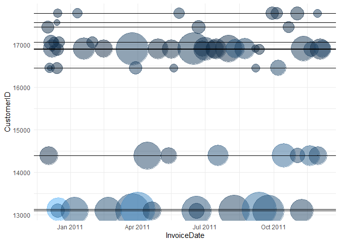
For random 10 customers, the total sales and number of items sold across time are shown in a bubble plot.

You can observe that there are gaps between purchases for different customers. 'Gap' is the difference in months between two successive purchases or the difference between the current month (despite no purchase) and the last purchase month. The frequency distribution of all the purchases at different gaps is shown below:

Cumulative frequency
gap_month	Count	cumsum
0	489	51.58228
1	108	62.97468
2	50	68.24895
3	33	71.72996
4	20	73.83966
5	30	77.00422
6	18	78.90295
7	18	80.80169
8	21	83.01688
9	6	83.64979
10	20	85.75949
11	38	89.76793
12	97	100.00000

From the above distribution, I am assuming that a customer who has not transacted for greater than 6 months is inactive.

Creating a Markov chain¶

Loading the libraries required in this section

At 2011-06-01, the state of a customer is given by:

elapsed_months <- function(end_date, start_date) {
    ed <- as.POSIXlt(end_date)
    sd <- as.POSIXlt(start_date)
    12 * (ed$year - sd$year) + (ed$mon - sd$mon)
}
final_classes <- filtered_data %>% filter(InvoiceDate < date('2011-07-01')) %>%
  group_by(CustomerID) %>% 
  summarise(recent_purchase_date = max(InvoiceDate)) %>% 
  mutate(Class1 = elapsed_months(date('2011-07-01'), date(recent_purchase_date))) %>% 
  mutate(Class1 = as.integer(Class1))
kable(final_classes %>% sample_n(10), align = 'c', caption = 'Initial state') %>% 
   kable_styling(full_width = F)

Initial state
CustomerID	recent_purchase_date	Class1
17450	2011-06-21 16:01:00	1
14896	2011-05-19 10:20:00	2
18061	2011-06-10 14:46:00	1
13065	2010-12-01 16:52:00	7
17231	2011-06-02 19:50:00	1
15894	2011-03-31 13:50:00	4
14729	2010-12-01 12:43:00	7
15965	2010-12-07 13:18:00	7
15834	2011-06-27 10:16:00	1
16081	2011-06-07 13:31:00	1

Here the states are defined as:

State	Recency Level	Explanation
1	1	Last purchase made this month
2	2	Last purchase made last month
3	3	Last purchase made 2 months ago
4	4	Last purchase made 3 months ago
5	5	Last purchase made 4 months ago
6	6	Last purchase made 5 months ago
7	7-12	Purchase made 6 months or before (Churn state)

Similarly, the state of the customer at the start of each month is:

States after every month
CustomerID	recent_purchase_date	Class1	Class2	Class3	Class4	Class5	Class6
13831	2011-05-23 13:25:00	2	1	2	1	2	1
12779	2011-06-03 10:37:00	1	2	3	4	5	1
17519	2011-06-19 13:55:00	1	1	2	3	4	1
12434	2011-04-04 09:57:00	3	4	5	1	2	3
13021	2011-06-26 11:53:00	1	1	2	1	2	1
17860	2010-12-06 12:41:00	7	7	7	7	7	7
12585	2011-04-19 13:39:00	3	4	5	6	7	7
16995	2010-12-02 17:09:00	7	7	7	7	7	7
14911	2011-06-30 15:46:00	1	1	1	1	1	1
15350	2010-12-01 13:33:00	7	7	7	7	7	7

I can observe that every customer moves from one class (state) to another state every month (step). According to Markov, the probability of a customer to move to state j at any step is only given by the previous state i. $$ P_{ij} = P(X_{t+1} = j | X_{t} = i) $$ For each interaction (Class1 to Class 2, month 2 to month 3, Step 3 to step 4), a transaction matrix can be created which has the probability of moving from i the state to j state.

But before I can create the one-step transition probabilities, I need to check whether the sequence of random variables can be approximated to a Markov chain. This is carried out using Anderson−Goodman test which is a chi-square test of independence.
The null and alternative hypotheses to check whether the sequence of random variables follows a Markov chain is stated below:
$H_0$: The sequences of transitions ($X_1, X_2, …, X_n$) are independent (zero-order Markov chain)
$H_A$: The sequences of transitions ($X_1, X_2, …, X_n$) are dependent (first-order Markov chain)
The corresponding test statistic is $$ \chi^2 = \sum_{i} \sum_{j} (\frac{(O_{ij} -E_{ij})^2}{E_{jj}}) $$

The transition probability matrix for the transition form State 1 to 2 is:

seq_matr <- markovchainFit(final_classes[3:4], method = "mle", name = 'CLV')
seq_matr$estimate

## CLV 
##  A  7 - dimensional discrete Markov Chain defined by the following states: 
##  1, 2, 3, 4, 5, 6, 7 
##  The transition matrix  (by rows)  is defined as follows: 
##            1         2         3    4         5         6         7
## 1 0.57777778 0.4222222 0.0000000 0.00 0.0000000 0.0000000 0.0000000
## 2 0.42957746 0.0000000 0.5704225 0.00 0.0000000 0.0000000 0.0000000
## 3 0.32000000 0.0000000 0.0000000 0.68 0.0000000 0.0000000 0.0000000
## 4 0.13461538 0.0000000 0.0000000 0.00 0.8653846 0.0000000 0.0000000
## 5 0.18181818 0.0000000 0.0000000 0.00 0.0000000 0.8181818 0.0000000
## 6 0.08333333 0.0000000 0.0000000 0.00 0.0000000 0.0000000 0.9166667
## 7 0.10800000 0.0000000 0.0000000 0.00 0.0000000 0.0000000 0.8920000

From the above matrix, P(4,5) = 0.8684211 means that the probability of moving from State 4 to State 5 is 86%. That means that a customer who has not purchased any item in 3 months has an 86% probability of not purchasing any item the next month also.

Similarly, the Transition matrix for all the steps is:

sequenceMatr = list()
for(i in 1:5){
  sequenceMatr[[i]] <- markovchainFit(final_classes[(2+i):(3+i)], method = "map")$estimate@transitionMatrix
}
sequenceMatr

## [[1]]
##            1         2         3    4         5         6         7
## 1 0.57777778 0.4222222 0.0000000 0.00 0.0000000 0.0000000 0.0000000
## 2 0.42957746 0.0000000 0.5704225 0.00 0.0000000 0.0000000 0.0000000
## 3 0.32000000 0.0000000 0.0000000 0.68 0.0000000 0.0000000 0.0000000
## 4 0.13461538 0.0000000 0.0000000 0.00 0.8653846 0.0000000 0.0000000
## 5 0.18181818 0.0000000 0.0000000 0.00 0.0000000 0.8181818 0.0000000
## 6 0.08333333 0.0000000 0.0000000 0.00 0.0000000 0.0000000 0.9166667
## 7 0.10800000 0.0000000 0.0000000 0.00 0.0000000 0.0000000 0.8920000
## 
## [[2]]
##            1         2         3         4         5         6         7
## 1 0.61309524 0.3869048 0.0000000 0.0000000 0.0000000 0.0000000 0.0000000
## 2 0.36184211 0.0000000 0.6381579 0.0000000 0.0000000 0.0000000 0.0000000
## 3 0.39506173 0.0000000 0.0000000 0.6049383 0.0000000 0.0000000 0.0000000
## 4 0.13725490 0.0000000 0.0000000 0.0000000 0.8627451 0.0000000 0.0000000
## 5 0.22222222 0.0000000 0.0000000 0.0000000 0.0000000 0.7777778 0.0000000
## 6 0.11111111 0.0000000 0.0000000 0.0000000 0.0000000 0.0000000 0.8888889
## 7 0.08984375 0.0000000 0.0000000 0.0000000 0.0000000 0.0000000 0.9101562
## 
## [[3]]
##           1         2         3         4         5         6         7
## 1 0.6220238 0.3779762 0.0000000 0.0000000 0.0000000 0.0000000 0.0000000
## 2 0.4769231 0.0000000 0.5230769 0.0000000 0.0000000 0.0000000 0.0000000
## 3 0.4020619 0.0000000 0.0000000 0.5979381 0.0000000 0.0000000 0.0000000
## 4 0.3877551 0.0000000 0.0000000 0.0000000 0.6122449 0.0000000 0.0000000
## 5 0.2727273 0.0000000 0.0000000 0.0000000 0.0000000 0.7272727 0.0000000
## 6 0.2000000 0.0000000 0.0000000 0.0000000 0.0000000 0.0000000 0.8000000
## 7 0.1011673 0.0000000 0.0000000 0.0000000 0.0000000 0.0000000 0.8988327
## 
## [[4]]
##           1         2         3         4         5         6         7
## 1 0.5828877 0.4171123 0.0000000 0.0000000 0.0000000 0.0000000 0.0000000
## 2 0.4566929 0.0000000 0.5433071 0.0000000 0.0000000 0.0000000 0.0000000
## 3 0.3823529 0.0000000 0.0000000 0.6176471 0.0000000 0.0000000 0.0000000
## 4 0.2586207 0.0000000 0.0000000 0.0000000 0.7413793 0.0000000 0.0000000
## 5 0.1333333 0.0000000 0.0000000 0.0000000 0.0000000 0.8666667 0.0000000
## 6 0.1875000 0.0000000 0.0000000 0.0000000 0.0000000 0.0000000 0.8125000
## 7 0.1042471 0.0000000 0.0000000 0.0000000 0.0000000 0.0000000 0.8957529
## 
## [[5]]
##           1         2         3         4         5         6         7
## 1 0.7118644 0.2881356 0.0000000 0.0000000 0.0000000 0.0000000 0.0000000
## 2 0.6666667 0.0000000 0.3333333 0.0000000 0.0000000 0.0000000 0.0000000
## 3 0.4492754 0.0000000 0.0000000 0.5507246 0.0000000 0.0000000 0.0000000
## 4 0.3095238 0.0000000 0.0000000 0.0000000 0.6904762 0.0000000 0.0000000
## 5 0.2790698 0.0000000 0.0000000 0.0000000 0.0000000 0.7209302 0.0000000
## 6 0.2307692 0.0000000 0.0000000 0.0000000 0.0000000 0.0000000 0.7692308
## 7 0.2170543 0.0000000 0.0000000 0.0000000 0.0000000 0.0000000 0.7829457

The Transition Probabilities at various steps seem to follow a pattern. I can do a likelihood ratio test to test the homogeneity of transition matrices. That means I want to find out if the changes in TP across time are random, and I can take a constant TP to describe the different TP's or not.
The Null and alternative hypothesis is:
$H_0 : P_{ij} (t) = P_{ij}$
$H_1 : P_{ij} (t) \neq P_{ij}$

The test statistic for a likelihood ratio test (Chi-square test) is given by $$ \chi^2 = \sum_{t} \sum_{i} \sum_{j} \frac{n(t)[\hat P_{ij}(t)-\hat P_{ij}]^2}{\hat P_{ij}} $$ where n(t) is the number of customers in state i at time t. The test statistic follows a $\chi^2$ distribution with (t − 1) × m × (m − 1) degrees of freedom.

verifyHomogeneity(sequenceMatr)

## Testing homogeneity of DTMC underlying input list 
## ChiSq statistic is 0.8694698 d.o.f are 192 corresponding p-value is 1

## $statistic
## [1] 0.8694698
## 
## $dof
## [1] 192
## 
## $pvalue
## [1] 1

As the p-value is greater than the $\alpha = 0.05$, I am retaining the Null hypothesis that the transition probabilities are homogeneous.

The final TP will be as follows:

finalTP <- sequenceMatr[[1]]
for(i in 2:5){
  finalTP <- finalTP+sequenceMatr[[i]]
}
finalTP <- finalTP/5
CLT.mc <- new('markovchain', 
                  # states = colnames(finalTP),
                  transitionMatrix = finalTP,
                  name = 'CLT')
CLT.mc

## CLT 
##  A  7 - dimensional discrete Markov Chain defined by the following states: 
##  1, 2, 3, 4, 5, 6, 7 
##  The transition matrix  (by rows)  is defined as follows: 
##           1         2         3         4        5         6         7
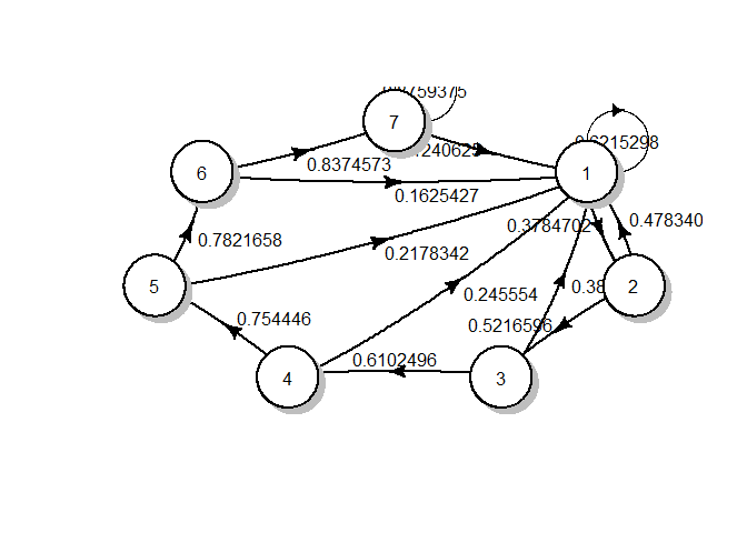
## 1 0.6215298 0.3784702 0.0000000 0.0000000 0.000000 0.0000000 0.0000000
## 2 0.4783404 0.0000000 0.5216596 0.0000000 0.000000 0.0000000 0.0000000
## 3 0.3897504 0.0000000 0.0000000 0.6102496 0.000000 0.0000000 0.0000000
## 4 0.2455540 0.0000000 0.0000000 0.0000000 0.754446 0.0000000 0.0000000
## 5 0.2178342 0.0000000 0.0000000 0.0000000 0.000000 0.7821658 0.0000000
## 6 0.1625427 0.0000000 0.0000000 0.0000000 0.000000 0.0000000 0.8374573
## 7 0.1240625 0.0000000 0.0000000 0.0000000 0.000000 0.0000000 0.8759375

The Markov chain can be visualized as follows:

plotmat(t(CLT.mc@transitionMatrix), box.size = 0.05)

The initial frequency of the classes are:

initial_freq <- (final_classes %>% group_by(Class1) %>% summarise(frequency = n()/nrow(final_classes)))$frequency
initial_freq

## [1] 0.37974684 0.14978903 0.07911392 0.05485232 0.03481013 0.03797468 0.26371308

As TP is the transition probability between states, I can find the number of people in each state at any time t using the following formula:

\[ u^{(n)} = uP^{(n)} \]

From the TP, the frequency in the first stage is compared with the actual frequency at the 1^st stage.

## # A tibble: 7 x 3
##   Class2 actual_frequency predicted_frequency
##    <dbl>            <dbl>               <dbl>
## 1      1           0.354               0.236 
## 2      2           0.160               0.0567
## 3      3           0.0854              0     
## 4      4           0.0538              0     
## 5      5           0.0475              0     
## 6      6           0.0285              0     
## 7      7           0.270               0

Similarly, for 3^rd stage

## # A tibble: 7 x 3
##   Class4 actual_frequency predicted_frequency
##    <dbl>            <dbl>               <dbl>
## 1      1           0.395               0.409 
## 2      2           0.134               0.153 
## 3      3           0.0717              0.0787
## 4      4           0.0612              0.0458
## 5      5           0.0316              0.0360
## 6      6           0.0338              0.0285
## 7      7           0.273               0.249

I can observe that a Markov chain can be used to find the number of people in each state after each stage. So the probability of people in each class after n steps is given below:

## [1] "n = 1"
##              1         2          3          4          5          6         7
## [1,] 0.3984503 0.1437229 0.07813888 0.04827924 0.04138312 0.02722729 0.2627984
## [1] "n = 14"
##              1         2          3          4         5          6         7
## [1,] 0.4260002 0.1610742 0.08392567 0.05113945 0.0385104 0.03005181 0.2092984
## [1] "n = 34"
##             1         2          3          4          5          6         7
## [1,] 0.427639 0.1618467 0.08442764 0.05152099 0.03886892 0.03040108 0.2052957
## [1] "n = 39"
##              1         2          3          4          5        6         7
## [1,] 0.4276527 0.1618532 0.08443183 0.05152418 0.03887192 0.030404 0.2052623
## [1] "n = 43"
##              1        2          3          4          5          6         7
## [1,] 0.4276567 0.161855 0.08443306 0.05152511 0.03887279 0.03040485 0.2052525
## [1] "n = 51"
##             1         2          3          4          5          6         7
## [1,] 0.427659 0.1618562 0.08443378 0.05152566 0.03887331 0.03040535 0.2052467
## [1] "n = 59"
##              1         2         3          4         5          6         7
## [1,] 0.4276594 0.1618563 0.0844339 0.05152575 0.0388734 0.03040544 0.2052457
## [1] "n = 68"
##              1         2          3          4          5          6         7
## [1,] 0.4276595 0.1618564 0.08443393 0.05152577 0.03887341 0.03040545 0.2052456
## [1] "n = 82"
##              1         2          3          4          5          6         7
## [1,] 0.4276595 0.1618564 0.08443393 0.05152577 0.03887341 0.03040546 0.2052455
## [1] "n = 87"
##              1         2          3          4          5          6         7
## [1,] 0.4276595 0.1618564 0.08443393 0.05152577 0.03887341 0.03040546 0.2052455

I can observe that as 'n' is increasing, the frequency of customers is tending towards constant. This constant is called steady state frequency. The steady state probability is :

steady.state.prob <- steadyStates(CLT.mc)
steady.state.prob

##              1         2          3          4          5          6         7
## [1,] 0.4276595 0.1618564 0.08443393 0.05152577 0.03887341 0.03040546 0.2052455

The probability change with steps can be visualized as below:

Customer Lifetime value¶

Now that I established that the customer segments can be represented as a Markov chain, I can compute the customer lifetime value.
The monetary value at each state is

revenue_in_states <- filtered_data %>% left_join(final_classes, by = 'CustomerID') %>%
  filter(InvoiceDate < date('2011-07-01')) %>%
  dplyr::select(Class1, total_sales) %>%
  group_by(Class1) %>%
  summarise(avg_revenue = mean(total_sales))
kable(revenue_in_states, align = 'c', caption = 'States after steps') %>% 
   kable_styling(full_width = F)

States after steps
Class1	avg_revenue
1	56.51656
2	56.17425
3	56.45380
4	44.33256
5	46.58667
6	49.00257
7	52.82802

The steady-state retention probability is given by $$ R_t = 1 - \frac{\pi_0(1-P_0)}{1-\pi_0}$$ Where $P_{00}$ is the transition probability of the null state (State 7), and $\pi_0$ is the steady state distribution of the Null state (State 7). Substituting I get:

## [1] 0.9679608

Similarly Customer lifetime value for 5 periods is given by:
$$ CLV = \sum_{t=0}^{5} \frac{P_I×P^t×R}{(1+i)t} $$ Where PI is the initial distribution of customers in different states, P is the transition probability matrix, R is the reward vector (margin generated in each customer segment). The interest rate is i (discount rate), $d = 1 + \frac{1}{1+i}=0.95$ is the discount factor.
Substituting, I get:

CLT <- 0
for(k in 0:5){
  CLT = CLT + (0.95^k)*(initial_freq %*% (CLT.mc@transitionMatrix^k) %*% revenue_in_states$avg_revenue)
}
CLT

##          [,1]
## [1,] 484.3484

Therefore, the customer lifetime value is 484.34.

References¶

Business Analytics: The Science of Data-Driven Decision Making Available
Introduction to probability, Charles M. Grinstead and J. Laurie Snell, Available
CS294 Markov Chain Monte Carlo: Foundations & Applications (lecture by Prof. Alistair Sinclair in Fall 2009) Available
Computer Science Theory for the Information Age, Spring 2012 (course material) Available
Customer Analytics at Flipkart.com Available
IIMB BAI Class notes and practice problems