CART Classification (R)
Decision Trees
Decision trees are a collection of predictive analytic techniques that use tree-like graphs for predicting the response variable. One such method is CHAID explained in a previous blog. The most popular decision tree method is the CART or the Classification and regression trees. Decision trees partition the data set into mutually exclusive and exhaustive subsets, which results in the splitting of the original data resembling a tree-like structure.
CART Classification
We can use the CART method for regression and classification. In this blog, I will go through the CART classification in detail using the titanic example. Any decision tree model consists of 5 steps:
1. Start with the complete training data in the root node.
2. Decide on a splitting criterion
3. Split the data into two or more subsets based on the above metric
4. Using independent variables, repeat step 3 for each of the subsets of the data until
--(a) All the dependent variables are exhausted, or they are not statistically significant at alpha
--(b) We meet the stopping criteria
5. Generate business rules for the terminal nodes (nodes without any branches) of the tree
Step 1: Start with complete data
The data used in this blog is the same as the used in other classification posts, i.e. the Titanic dataset from Kaggle. In this problem, we have to identify what types of people had a higher chance of survival. A sample of the data is shown below. A basic EDA is performed in the blog on Logistic regression.
| Survived | Pclass | Sex | Age | SibSp | Parch | Fare | Embarked |
|---|---|---|---|---|---|---|---|
| I | 3 | female | 14 | 1 | 0 | 11.2417 | C |
| O | 2 | male | 21 | 1 | 0 | 11.5000 | S |
| I | 2 | female | 24 | 0 | 2 | 14.5000 | S |
| I | 2 | female | 29 | 0 | 0 | 10.5000 | S |
| O | 1 | male | 27 | 0 | 2 | 211.5000 | C |
Step 2: Decide on a splitting criterion
In CHAID bases classification, we used p-value from hypothesis tests as the splitting criterion. In CART, we will use impurity metrics like Gini Index and Entropy.
Gini Index
It is defined mathematically as: $$ Gini\,Index = \sum_{i=1}^k \sum_{j=1,i\neq 1}^k P(C_i|t)\times P(C_j|t)$$ where \(P(C_i|t)\) = Proportion of observations belonging to class \(C_i\) in node t. For a binary classification,
Gini Index is a measure of total variance across the classes. It has a small value if all the \(P(C_i|t)\) are close to zero or one. For this reason, the Gini index is a measure of node purity. A small value indicates that a node contains observations from a single class predominantly.
Entropy
An alternative to the Gini index is entropy, given by entropy: $$ Entropy = - \sum_{i=1}^k P(C_i|t)\times log[P(C_i|t]$$ Like the Gini index, the entropy is a small value if the node is pure. The Gini index and the entropy are quite similar numerically.
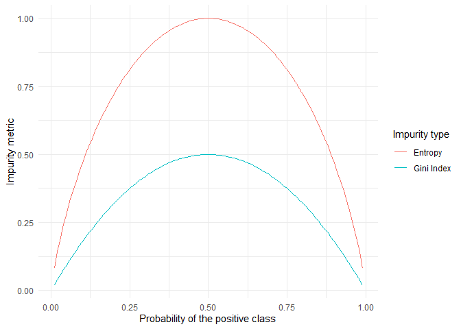
For this blog, I want to consider the Gini index as my impurity measure. The aim is to minimise the Gini Index as much as possible.
Step 3. Split the data into two or more subsets based on the above metric
The Gini impurity in the base node (complete data) is
## [1] 0.472365
The impurity of the overall data is 0.47. Let us look at the purity if we split the data based on various features.
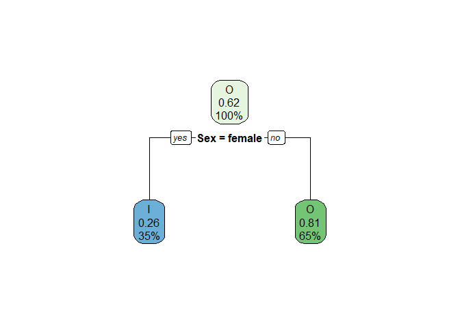
Gender:
If we split based on gender, the male and female branches individually have lower impurity (Gini index) than the base node. I have built the decision tree as the total weighted Gini index after splitting is lesser than the Gini index of the overall data.
| Var1 | I | O | proportion.of.obs | child.gini.index |
|---|---|---|---|---|
| female | 231 | 81 | 0.3509561 | 0.3844305 |
| male | 109 | 468 | 0.6490439 | 0.3064437 |
## [1] "The total weighted impurity after the split is: 0.3338"
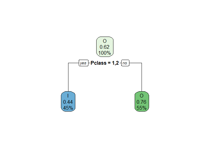
Passenger class
Similarly, for passenger class, the three categories (if we split into three branches) have an impurity as follows:
| Var1 | I | O | proportion.of.obs | child.gini.index |
|---|---|---|---|---|
| 1 | 134 | 80 | 0.2407199 | 0.4681632 |
| 2 | 87 | 97 | 0.2069741 | 0.4985232 |
| 3 | 119 | 372 | 0.5523060 | 0.3672459 |
In CART, we can split the data into two branches only. By combining passenger class 1 and passenger class 2 into one category, we will have the below Gini impurities. I have built the decision tree as the total weighted Gini index after splitting is lesser than the Gini index of the overall data.
| Var1 | I | O | proportion.of.obs | child.gini.index |
|---|---|---|---|---|
| 3rd Class | 119 | 372 | 0.552306 | 0.3672459 |
| First and second Class | 221 | 177 | 0.447694 | 0.4938890 |
## [1] "The total weighted impurity after the split is: 0.423943259996532"
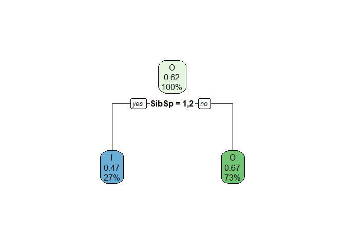
Number of siblings
The number of siblings is a categorical variable in this problem as the probability of survival is not linearly dependent on the number of siblings. According to intuition, people with one or two siblings will have a higher rate of survival as they will take care of each other. The impurity for each class is:
| Var1 | I | O | proportion.of.obs | child.gini.index |
|---|---|---|---|---|
| 0 | 208 | 398 | 0.6816648 | 0.4508490 |
| 1 | 112 | 97 | 0.2350956 | 0.4974245 |
| 2 | 13 | 15 | 0.0314961 | 0.4974490 |
| 3 | 4 | 12 | 0.0179978 | 0.3750000 |
| 4 | 3 | 15 | 0.0202475 | 0.2777778 |
| 5 | 0 | 5 | 0.0056243 | 0.0000000 |
| 8 | 0 | 7 | 0.0078740 | 0.0000000 |
By combining the number of siblings of 1 and 2 into one category and all others into another group, we will have the following Gini index:
| Var1 | I | O | proportion.of.obs | child.gini.index |
|---|---|---|---|---|
| One or two siblings | 125 | 112 | 0.2665917 | 0.4984956 |
| others | 215 | 437 | 0.7334083 | 0.4420330 |
## [1] "The total weighted impurity after the split is: 0.457085468377958"
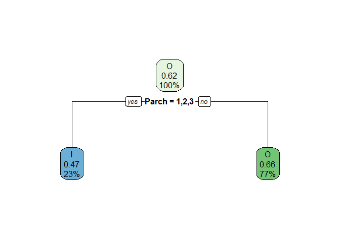
Number of parents/children
Just like the number of siblings, the number of parents/children of a person is also a categorical variable. The Gini index among the categories are:
| Var1 | I | O | proportion.of.obs | child.gini.index |
|---|---|---|---|---|
| 0 | 231 | 445 | 0.7604049 | 0.4498923 |
| 1 | 65 | 53 | 0.1327334 | 0.4948291 |
| 2 | 40 | 40 | 0.0899888 | 0.5000000 |
| 3 | 3 | 2 | 0.0056243 | 0.4800000 |
| 4 | 0 | 4 | 0.0044994 | 0.0000000 |
| 5 | 1 | 4 | 0.0056243 | 0.3200000 |
| 6 | 0 | 1 | 0.0011249 | 0.0000000 |
By combining the number of parents/siblings of 1, 2 and 3 into one group and others into another group, we will have the following impurity:
| Var1 | I | O | proportion.of.obs | child.gini.index |
|---|---|---|---|---|
| 1,2&3 | 108 | 95 | 0.2283465 | 0.4979495 |
| others | 232 | 454 | 0.7716535 | 0.4476366 |
## [1] "The total weighted impurity after the split is: 0.459125378001722"
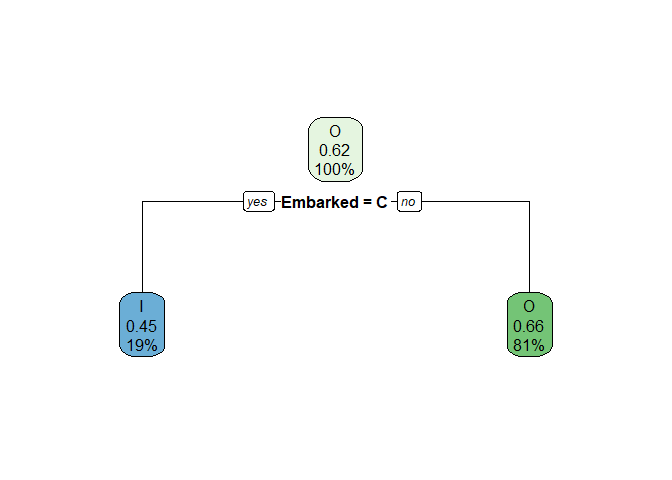
Embarked location
There are three locations where the passengers have embarked. The Gini index within each of the location is:
| Var1 | I | O | proportion.of.obs | child.gini.index |
|---|---|---|---|---|
| C | 93 | 75 | 0.1889764 | 0.4942602 |
| Q | 30 | 47 | 0.0866142 | 0.4756283 |
| S | 217 | 427 | 0.7244094 | 0.4468336 |
Combining Q and S into one category, we have:
| Var1 | I | O | proportion.of.obs | child.gini.index |
|---|---|---|---|---|
| C | 93 | 75 | 0.1889764 | 0.4942602 |
| Q&S | 247 | 474 | 0.8110236 | 0.4504377 |
## [1] "The total weighted impurity after the split is: 0.458719142423424"
Age
Age is a continuous variable, so we have to find the ideal age to split the data along with the impurity metrics. To find the ideal cutoff, I have plotted the weighted gini index for split based on different ages. 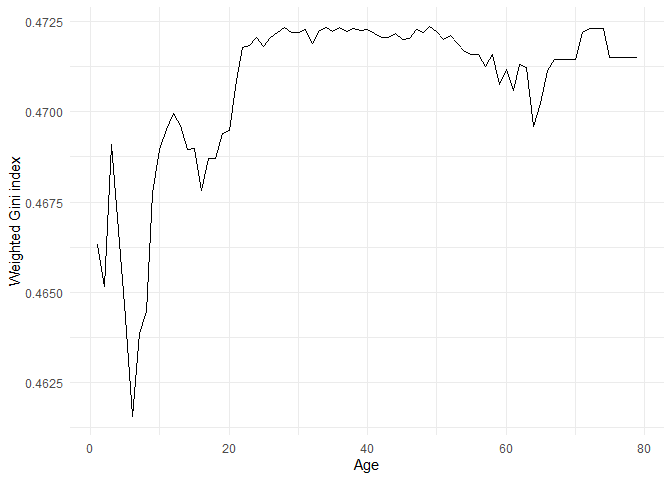
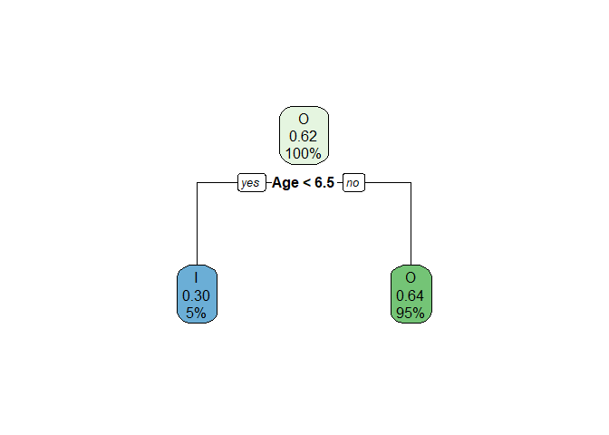
We can observe the minimum Gini index when the data is split at Age=7 years.
| Age_class | survived_prob | proportion.of.obs | child.gini.index |
|---|---|---|---|
| <7 | 0.6470588 | 0.0573678 | 0.4567474 |
| >=7 | 0.3663484 | 0.9426322 | 0.4642745 |
## [1] "The total weighted impurity after the split is: 0.46"
Fare
Similar to age, fare is a continuous variable and we have to find the optimal fare to split first.
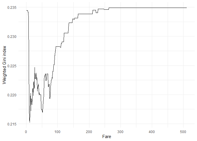
The optimal fare is 11. The impurity metrics for this split are:
| Fare_class | survived_prob | proportion.of.obs | child.gini.index |
|---|---|---|---|
| <=11 | 0.2087912 | 0.4094488 | 0.3303949 |
| >11 | 0.5028571 | 0.5905512 | 0.4999837 |
Conclusion
Among all the factors above, Gender has the least Gini Index of 0.3338. So the initial split of the data would be on Gender.
Step 4: Repeat step 3 until stopping criterion
After splitting the data based on gender, we will get two data sets. We should perform a similar analysis to step 2 to split the data further, and so on. The splitting should stop when we meet the stopping criterion. Different stopping criterion for CART classification trees are:
1. The number of cases in the node is less than some pre-specified limit.
2. The purity of the node is more than some pre-specified threshold.
3. Depth of the node is more than some pre-specified threshold.
4. Predictor values for all records are identical
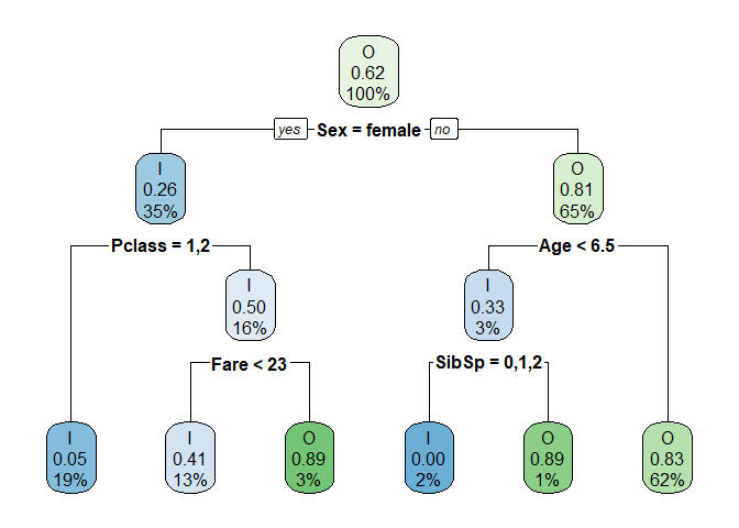
In this blog, I want to give a maximum depth of trees as 3. In the machine learning blogs, I will go deeper into how to select ideal stopping criterion. For max depth=3, we get the following decision tree:
Step 5: Making business rules
From the above tree, I can see generate the following rules:
1. A female passenger has a higher probability of surviving unless she is travelling in third class with a fare less than 23.
2. A male passenger has a lower likelihood of surviving unless he is a child of age less than six years and with up to two siblings.
Using this decision tree, we can observe how sociological factors like gender, age and monetary status affected the decisions on who would get into a lifeboat at a crucial time during the titanic disaster.