ARIMA in R

Arima model¶

ARIMA, short for 'Auto Regressive Integrated Moving Average' is a very popular forecasting model. ARIMA models are basically regression models: auto-regression simply means regression of a variable on itself measured at different time periods.

AR: Autoregression. A model that uses the dependent relationship between an observation and some number of lagged observations
I: Integrated. The use of differencing of raw observations (i.e. subtracting an observation from an observation at the previous time step) in order to make the time series stationary
MA: Moving Average. A model that uses the dependency between an observation and residual errors from a moving average model applied to lagged observations

Stationary¶

The assumption of AR model is that the time series is assumed to be a stationary process. If a time-series data, $Y_t$, is stationary, then it satisfies the following conditions:
1. The mean values of $Y_t$ at different values of t are constant
2. The variances of $Y_t$ at different time periods are constant (Homoscedasticity)
3. The covariances of $Y_t$ and $Y_{t-k}$ for different lags depend only on k and not on time t

Box-Jenkins method¶

The initial ARMA and ARIMA models were developed by Box and Jenkins in 1970. The authors also suggested a process for identifying, estimating, and checking models for any specific time series data-set. It contains three steps

Model form selection
1.1 Evaluate stationarity
1.2 Selection of the differencing level (d) – to fix stationarity problems
1.3 Selection of the AR level (p)
1.4 Selection of the MA level (q)
Parameter estimation
Model checking

Model form selection¶

Evaluate stationarity¶

A stationary time series is one whose properties do not depend on the time at which the series is observed. Time series with trends, or with seasonality, are not stationary. A white noise series is stationary — it does not matter when you observe it, it should look much the same at any point in time.

The presence of stationarity can be found in many ways among which the most popular three are:
1. ACF plot: When the data is non-stationary, the auto-correlation function will not be cut-off to zero quickly
2. Dickey−Fuller or augmented Dickey−Fuller tests
3. KPSS test

In the below example, I will use a sample from my attendance data set described in EDA blogs. (Actual data is not shown for privacy reasons. This is mock data which is very similar to the actual one. The analysis will be the same)

The time plot for the same is shown below: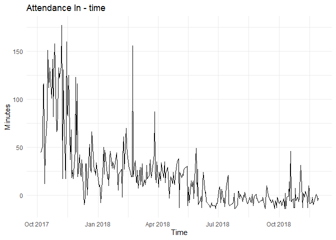

By looking at the plot, I can clearly see that the series is not stationary as the trend is visible and variance seems to be decreasing with time.
The ACF of this time series is:

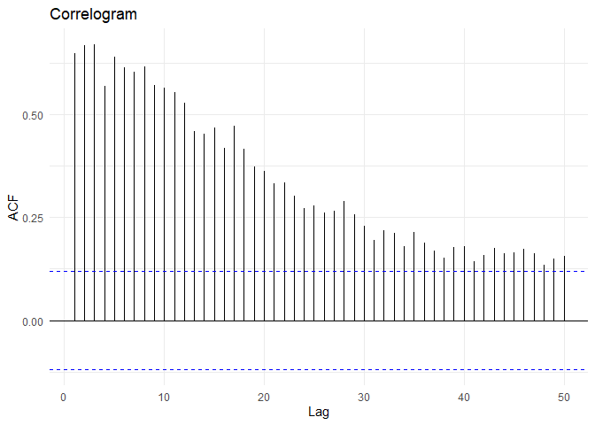
From the above plot, I can identify that the time series is not stationary.

Augmented Dickey−Fuller Test¶

Augmented Dickey−Fuller test is a hypothesis test in which the null hypothesis and alternative hypothesis are given by
$H_0$: $\gamma$ = 0 (the time series is non-stationary)
$H_1$: $\gamma$ < 0 (the time series is stationary)
Where $\Delta y_t = \alpha + \beta t + \gamma y_{t-1} + \delta_1 \Delta y_{t-1} + \delta_2 \Delta y_{t-2} + \dots$

## 
##  Augmented Dickey-Fuller Test
## 
## data:  time.series
## Dickey-Fuller = -2.8819, Lag order = 6, p-value = 0.2045
## alternative hypothesis: stationary

As p value is greater than the cut-off $ \alpha = 5\% $, retaining the null hypothesis that the time series is non-stationary.

KPSS Test¶

The null hypothesis for the KPSS test is that the data are stationary. For this test, we do NOT want to reject the null hypothesis.

## 
##  KPSS Test for Trend Stationarity
## 
## data:  time.series
## KPSS Trend = 0.41839, Truncation lag parameter = 5, p-value = 0.01

As p-value is less than 5%, rejecting the null hypothesis that the data is stationary.

Selection of differencing parameter d¶

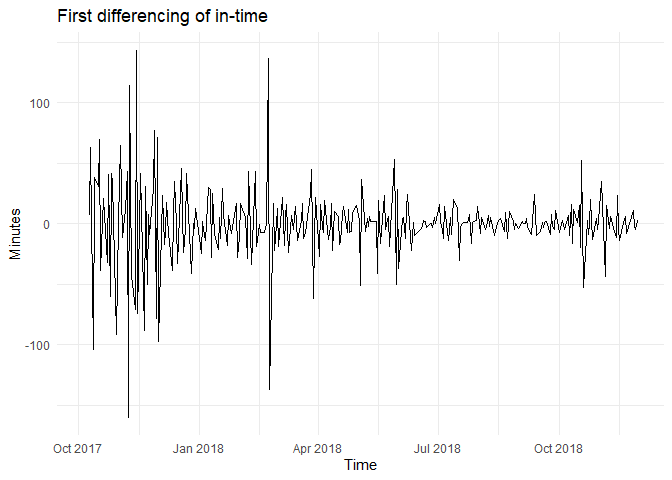
The attendance data (in time) have failed both tests for the stationary, the Augmented Dickey-Fuller and the KPSS test. Differencing is used to convert the data to a stationary model. Differencing is nothing but computing the differences between consecutive observations.

The above tests for first difference for in-time looks like the following:

## 
##  Augmented Dickey-Fuller Test
## 
## data:  time.series.diff
## Dickey-Fuller = -10.851, Lag order = 6, p-value = 0.01
## alternative hypothesis: stationary

## 
##  KPSS Test for Trend Stationarity
## 
## data:  time.series %>% diff()
## KPSS Trend = 0.01895, Truncation lag parameter = 5, p-value = 0.1

After differencing by d = 1, The ACF of the differenced in-time looks just like that of a white noise series. In the ADF test the p-value is lower than cut-off rejecting the Null hypothesis that time series is non-stationary while the KPSS test p-value is greater than 5% retaining the null hypothesis that the data is stationary. This suggests that after differencing by one time, the in-time is essentially a random amount and is stationary.

## [1] "The ideal differencing parameter is 1"

## 
## ####################### 
## # KPSS Unit Root Test # 
## ####################### 
## 
## Test is of type: mu with 5 lags. 
## 
## Value of test-statistic is: 0.0188 
## 
## Critical value for a significance level of: 
##                 10pct  5pct 2.5pct  1pct
## critical values 0.347 0.463  0.574 0.739

Selection of AR(p) and MA(q) parameters¶

One of the important tasks in using autoregressive model in forecasting is the model identification, which is, identifying the value of p and q (the number of lags).
Selection of AR(p) and MA(q) lags can be done by two methods:
1. ACF and PACF functions
2. AIC or BIC coefficients

ACF and PACF coefficients¶

Auto-correlation is the correlation between $Y_t$ measured at different time periods (for example, $Y_t$ and $Y_{t-1}$ or $Y_t$ and $Y_{t-k}$). A plot of auto-correlation for different values of k is called auto-correlation function (ACF) or correlogram.
Partial auto-correlation of lag k is the correlation between $Y_t$ and $Y_{t-k}$ when the influence of all intermediate values ($Y_{t-1}$, $Y_{t-2}$...$Y_{t-k+1}$) is removed (partial out) from both $Y_t$ and $Y_{t-k}$. A plot of partial auto-correlation for different values of k is called partial auto-correlation function (PACF).

Hypothesis tests can be carried out to check whether the auto-correlation and partial auto-correlation values are different from zero. The corresponding null and alternative hypotheses are
$H_0: r_k = 0$ and
$H_A: r_k \neq 0$,
where $r_k$ is the auto-correlation of order k

$H_0: r_{pk} = 0$ and
$H_A: r_{pk} \neq 0$,
where $r_{pk}$ is the partial auto-correlation of order k

The null hypothesis is rejected when $|r_k| > \frac{1 96}{\sqrt{n}}$ and $|r_{pk}| > \frac{1 96}{\sqrt{n}}$. In the ACF and PACF plots, this cut-off is shown as dotted blue lines.

The values of p and q in a ARMA process can be identified using the following thumb rule:
1. Auto-correlation value, $r_p > cutoff$ for first q values (first q lags) and cuts off to zero
2. Partial auto-correlation function, $r_{pk} > cutoff$ for first p values and cuts off to zero

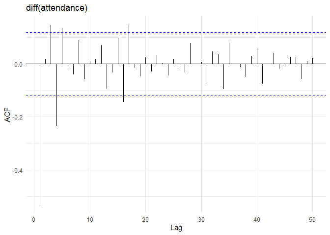
After differencing, the ACF and PACF plots of in0time are as follows: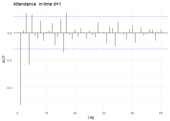

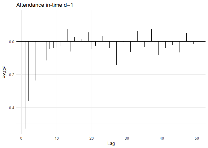
From the ACF and PACF plots. The auto-correlations cuts off to zero after the first lag. The PACF value cuts off to zero after 2 lags. So, the appropriate model could be ARMA(2, 1) process. Combining differencing parameter from previous section (d=1), The most appropriate model would be ARIMA(2, 1, 1)

AIC and BIC coefficients¶

Akaike’s Information Criterion (AIC) and Bayesian Information Criterion (BIC), which were useful in selecting predictors for regression, are also useful for determining the order of an ARIMA model. Best estimates of AR and MA orders will minimize AIC or BIC.

## 
##  Fitting models using approximations to speed things up...
## 
##  ARIMA(2,1,1) with drift         : 2503.652
##  ARIMA(0,1,0) with drift         : 2656.365
##  ARIMA(1,1,0) with drift         : 2569.569
##  ARIMA(0,1,1) with drift         : 2511.579
##  ARIMA(0,1,0)                    : 2654.343
##  ARIMA(1,1,1) with drift         : 2510.969
##  ARIMA(2,1,0) with drift         : 2526.337
##  ARIMA(3,1,1) with drift         : 2506.575
##  ARIMA(3,1,0) with drift         : 2523.835
##  ARIMA(2,1,1)                    : 2504.125
## 
##  Now re-fitting the best model(s) without approximations...
## 
##  ARIMA(2,1,1) with drift         : 2516.48
## 
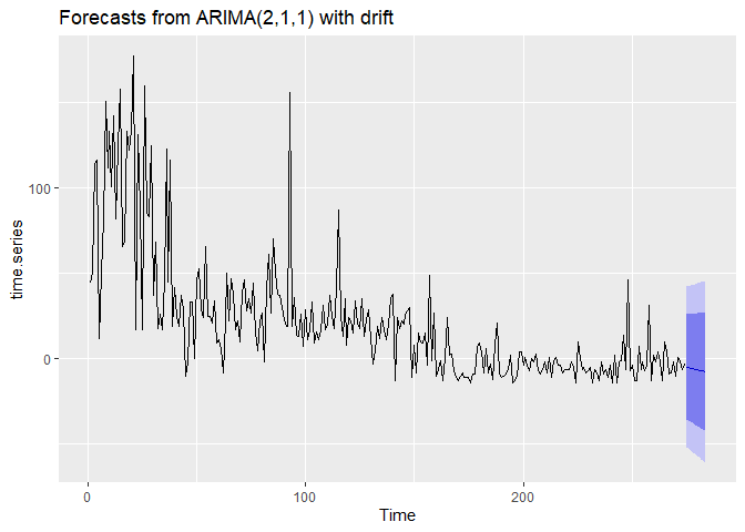
##  Best model: ARIMA(2,1,1) with drift

## Series: time.series 
## ARIMA(2,1,1) with drift 
## 
## Coefficients:
##           ar1     ar2      ma1    drift
##       -0.0530  0.0200  -0.8174  -0.3120
## s.e.   0.0811  0.0751   0.0539   0.2595
## 
## sigma^2 estimated as 574.2:  log likelihood=-1253.13
## AIC=2516.26   AICc=2516.48   BIC=2534.3

The model selected using AIC coefficient is ARIMA(2,1,1) which is same as the one selected using ACF and PACF.

ARIMA(2, 1, 1) is the final model as selected from both the methods.

Parameter estimation¶

Once the model order has been identified (i.e., the values of p, d and q), we need to estimate the model parameters. Using a regression model to identify the parameters:

## Series: time.series 
## ARIMA(2,1,1) with drift 
## 
## Coefficients:
##           ar1     ar2      ma1    drift
##       -0.0530  0.0200  -0.8174  -0.3120
## s.e.   0.0811  0.0751   0.0539   0.2595
## 
## sigma^2 estimated as 574.2:  log likelihood=-1253.13
## AIC=2516.26   AICc=2516.48   BIC=2534.3

Model testing¶

Residuals¶

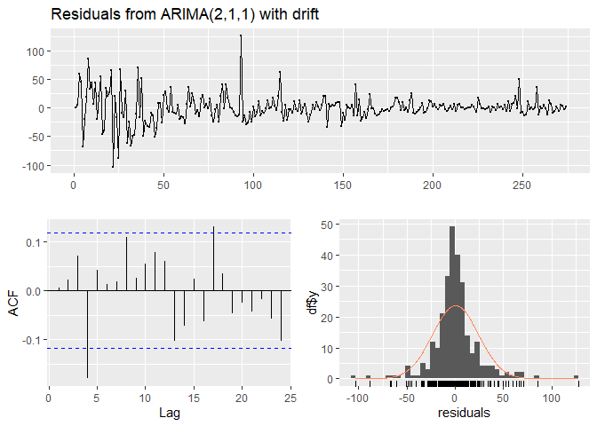
The “residuals” in a time series model are what is left over after fitting a model. Residuals are useful in checking whether a model has adequately captured the information in the data. A good forecasting method will yield residuals with the following properties:
1. The residuals are uncorrelated. If there are correlations between residuals, then there is information left in the residuals which should be used in computing forecasts.
2. The residuals have zero mean. If the residuals have a mean other than zero, then the forecasts are biased.

Portmanteau tests for auto-correlation¶

When we look at the ACF plot to see whether each spike is within the required limits, we are implicitly carrying out multiple hypothesis tests, each one with a small probability of giving a false positive. When enough of these tests are done, it is likely that at least one will give a false positive, and so we may conclude that the residuals have some remaining auto-correlation, when in fact they do not.

In order to overcome this problem, we test whether the first h auto-correlations are significantly different from what would be expected from a white noise process. A test for a group of auto-correlations is called a portmanteau test. One such test is the Ljung-Box test.

Ljung−Box Test for Auto-Correlations¶

Ljung−Box is a test of lack of fit of the forecasting model and checks whether the auto-correlations for the errors are different from zero. The null and alternative hypotheses are given by
$H_0$: The model does not show lack of fit
$H_1$: The model exhibits lack of fit
The Ljung−Box statistic (Q-Statistic) is given by $$ Q(m) = n(n+2) \sum_{k=1}^{{m}\frac{\rho_k}2}{n-k} $$ where n is the number of observations in the time series, k is the number of lag, $r_k$ is the auto-correlation of lag k, and m is the total number of lags. Q-statistic is an approximate chi-square distribution with m – p – q degrees of freedom where p and q are the AR and MA lags.

## 
##  Ljung-Box test
## 
## data:  Residuals from ARIMA(2,1,1) with drift
## Q* = 15.754, df = 6, p-value = 0.01513
## 
## Model df: 4.   Total lags used: 10

From the above tests we can conclude that the model is a good fit of the data.

References¶

Business Analytics: The Science of Data-Driven Decision Making - Dinesh Kumar
Forecasting: Principles and Practice - Rob J Hyndman and George Athanasopoulos - Online
SAS for Forecasting Time Series, Third Edition - Dickey
Applied Time Series Analysis for Fisheries and Environmental Sciences - E. E. Holmes, M. D. Scheuerell, and E. J. Ward - Online
The Box-Jenkins Method - NCSS Statistical Software - Online
Box-Jenkins modelling - Rob J Hyndman - Online
Basic Ecnometrics - Damodar N Gujarati
Time Series Analysis: Forecasting and Control - Box and Jenkins