The math behind ANN
Introduction
This is second in the series of blogs about neural networks. In this blog, we will discuss the back propagation algorithm. In the previous blog, we have seen how a single perceptron works when the data is linearly separable. In this blog, we will look at the working of a multi-layered perceptron (with theory) and understand the maths behind back propagation.
Multi-layer perceptron
An MLP is composed of one input layer, one or more layers of perceptrons called hidden layers, and one final perceptron layer called the output layer. Every layer except the input layer is connected with a bias neuron and is fully connected to the next layer.
Perceptron
In the previous blog, we have seen a perceptron with a single TLU. A Perceptron with two inputs and three outputs is shown below. Generally, an extra bias feature is added as input. It represents a particular type of neuron called bias neuron. A bias neuron outputs one all the time. This layer of TLUs is called a perceptron.
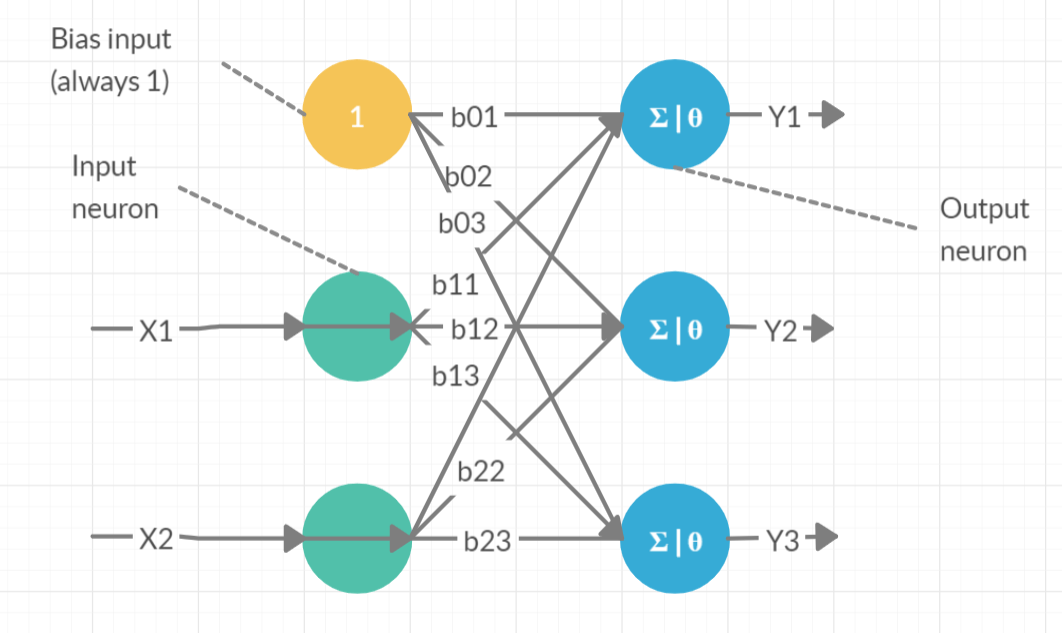
In the above perceptron, the inputs are x1 and x2. The outputs are y1, y2 and y3. Θ (or f) is the activation function. In the last blog, the step function is taken as the activation function. There are other activation functions such as:
Sigmoid function: It is S-shaped, continuous and differentiable where the output ranges from 0 to 1.
$$ f(z)=\frac{1}{1+e^{-z}} $$
Hyperbolic Tangent function: It is S-shaped, continuous and differentiable where the output ranges from -1 to 1. $$ f\left(z\right)=Tanh\left(z\right) $$
Training
Training a network in ANN has three stages, feedforward of input training pattern, back propagation of the error and adjustment of weights. Let us understand it using a simple example.
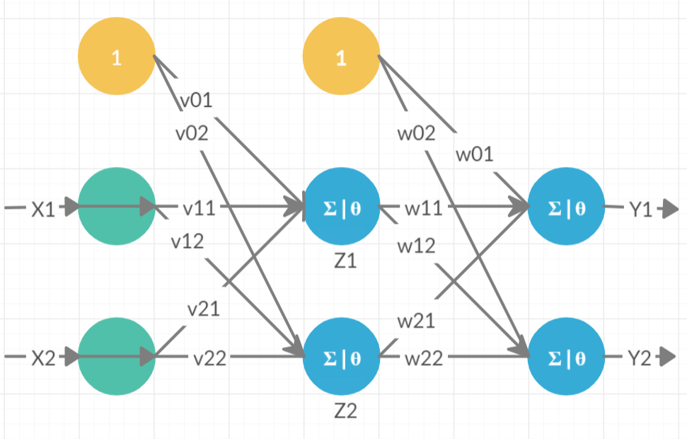
Consider a simple two-layered perceptron as shown:
Nomenclature
| Symbol | Meaning | Symbol | Meaning |
|---|---|---|---|
| \(X_i\) | Input | neuron | \(Y_k\) |
| \(x_i\) | Input value | \(y_k\) | Output value |
| \(Z_j\) | Hidden neuron | \(z_j\) | The output of a hidden neuron |
| \(\delta_k\) | The portion of error correction for weight \(w_{jk}\) | \(\delta_j\) | The portion of error correction for weight \(v_{ij}\) |
| \(w_{jk}\) | Weight of j to k | \(v_{ij}\) | weight of i to j |
| \(\alpha\) | Learning rate | \(t_j\) | Actual output |
| f | Activation function | -- | -- |
-
During feedforward, each input unit \(X_i\) receives input and broadcasts the signal to each of the hidden units \(Z_1\ldots Z_j\). Each hidden unit then computes its activation and sends its signal (\(z_j\)) to each output unit. Each output unit \(Y_k\) computes its activation (\(y_k\)) to form the response to the input pattern.
-
During training, each output unit \(Y_k\) compares its predicted output \(y_k\) with its actual output \(t_k\) to determine the error associated with that unit. Based on this error, \(\delta_k\) is computed. This \(\delta_k\) is used to distribute the error at the output unit back to all input units in the previous layers. Similarly, \(\delta_j\) is computed for all hidden layers \(Z_j\) which is propagated to the input layer.
-
The \(\delta_k\) and \(\delta_j\) are used to update the weights \(w_{jk}\) and \(v_{ij}\) respectively. The weight adjustment is based on gradient descent and is dependent on error gradient (\(\delta\)), learning rate (\(\alpha\)) and input to the neuron.
Mathematically this means the following:
Feedforward loop
- Each input unit (\(X_i\)) receives the input \(x_i\) and broadcasts this signal to all units to the hidden layers \(Z_j\).
Hidden layer
-
Each hidden unit (\(Z_j\)) sums its weighted input signals \(z\_in_j=v_{0j}+\sum_{i} x_i\times v_{ij}\)
-
The activation function is applied to this weighted sum to get the output. \(z_j=f\left(z\_in_j\right)\) (where f is the activation function).
-
Each hidden layer sends this signal (\(z_j\)) to the output layers.
Output layer
-
Each output unit (\(Y_k\)) sums its weighted input signals \(y\_in_k=w_{0k}+\sum_{j}z_j\times w_{jk}\)
-
The activation function is applied to this weighted sum to get the output. \(y_k=f\left(y\_in_k\right)\) (where f is the activation function).
Back propagation of error
Output layer
- The error information term (\(\delta_k\)) is computed at every output unit (\(Y_k\)). $$ \delta_k=\left(t_k-y_k\right)f’ y_in_k $$
- This error is propagated back to the hidden layer. (later weights will be updated using this \(\delta\))
Hidden layer
- Each hidden unit (\(Z_j\)) sums its weighted error from the output layer $$ \delta_in_j=\sum_{k}\delta_k\times w_{jk} $$
- The derivative of the activation function is multiplied to this weighted sum to get the weighted error information term at the hidden layer. $$ \delta_j=\delta_in_j \times f^\prime\left(z_in_j\right) $$ (where f is the activation function).
- This error is propagated back to the initial layer.
Update weights and biases
- The weights are updated based on the error information terms $$ w_{jk}\left(new\right)=w_{jk}\left(old\right)+\Delta w_{jk} $$ where $ \Delta w_{jk}=\alpha\times\delta_k\times z_j $
$$ v_{ij}\left(new\right)=v_{ij}\left(old\right)+\Delta v_{ij} $$ where $ \Delta v_{ij}=\alpha\times\delta_j\times x_i $
Steps 1 to 12 are done for each training epoch until a stopping criterion is met.
Derivation of learning rules
In every loop while training, we are changing the weights (\(v_{ij}\) and \(w_{jk}\)) to find the optimal solution. What we want to do is to find the effect of changing the weights on the error, and minimise the error using gradient descent.
The error gradient that has to be minimised is given by: $$ E=\frac{1}{2}\sum_{k}\left(t_k-y_k\right)^2 $$ The effect of changing an outer layer weight (\(w_{jk}\)) on the error is given by: $$ \frac{\partial E}{\partial w_{jk}}=\frac{\partial}{\partial w_{jk}}\frac{1}{2}\sum_{k}\left(t_k-y_k\right)^2 $$ $$ =\left(y_k-t_k\right)\frac{\partial}{\partial w_{jk}}f\left(y_in_k\right) $$ $$ =\left(y_k-t_k\right)\times z_j\times f'\left(y_in_k\right) $$ Therefore $$ \Delta w_{jk}=\alpha\frac{\partial E}{\partial w_{jk}}=\alpha\times\left(y_k-t_k\right)\times z_j\times f^\prime\left(y_in_k\right)={\alpha\times\delta}_k\times z_j $$
The effect of changing the weight of a hidden layer weight (\(v_{ij}\)) on the error is given by:
$$ \frac{\partial E}{\partial v_{ij}}=\sum_{k}{\left(y_k-t_k\right)\frac{\partial}{\partial v_{ij}}f\left(y_k\right)} $$ $$ =\sum_{k}\left(y_k-t_k\right)f^\prime\left(y_in_k\right)\frac{\partial}{\partial v_{ij}}f\left(y_k\right) $$ $$ =\sum_{k}\delta_kf^\prime\left(z_in_j\right)\left[x_i\right] =\delta_j\times x_i $$ Therefore $$ \Delta v_{ij}=\alpha\frac{\partial E}{\partial v_{ij}}={\alpha\times\delta}_j\times x_i $$ This way, for any number of layers, we can find the error information terms. Using gradient descent, we can minimise the error and find optimal weights for the ANN. In the next blog, we will implement ANN on the Titanic problem and compare it with logistic regression.
Reference
Fausett, L., 1994. Fundamentals of neural networks: architectures, algorithms, and applications. Prentice-Hall, Inc.