Collaborative Filtering (Python)
Neural collaborative filtering
Recommending music is common in music-based apps like NetEase or Spotify. This blog uses the data of 10k users (taken randomly) from the NetEase dataset to increase the click-through rate on the music cards (similar to TikTok/Instagram reels) recommended to the users. Recommending trending music to each unique user can decrease the chances of the user being inactive and increases the time spent by a user on the app.
Collaborative filtering creates item and user embeddings to understand the behaviour of different users and items. Neural Collaborative Filtering is modified to incorporate these other features as we have additional content-based and user-based features. This approach can use the power of collaborative filtering to create user and item embeddings independently and, simultaneously, use the additional content and user-based features given in the data for building the model.
import pandas as pd
import datetime
import numpy as np
import random
import warnings
warnings.filterwarnings('ignore')
The data for the most recent day the user has interacted is taken as a test set, while the rest is used for training the data. (The pre-processing of the dataset is not shown in this blog). The description of the data can be found in the paper NetEase Cloud Music Data and NetEase Cloud Dataset: Active User Identification and Deep Neural Network Based CTR.
# data is taken from end of part 1
train_data = pd.read_csv('train_data_10k.csv')
test_data = pd.read_csv('test_data_10k.csv')
For building a more robust recommendation system, we consider users with more than one click (already active users) and content with more than one click (popular content).
selected_users = test_data.userId.unique()

seen_mlogs = train_data.groupby('mlogId').userId.nunique().reset_index()
selected_mlogs = seen_mlogs[seen_mlogs.userId>1].mlogId.reset_index().mlogId

# filtering the data for the selected mlogs that have atleast one view
train_data = train_data[train_data.mlogId.isin(selected_mlogs)]

users_clicked = train_data[train_data.isClick == 1].groupby('userId').mlogId.nunique().reset_index()
selected_users = users_clicked[users_clicked.mlogId > 1].userId.reset_index().userId
train_data = train_data[train_data.userId.isin(selected_users)].reset_index()
The total number of users considered for the model
len(train_data.userId.unique())
719
Filtering the test data for the same users
test_data = test_data[test_data.userId.isin(selected_users)]
test_data = test_data[test_data.mlogId.isin(selected_mlogs)]
test_data = test_data.reset_index()
The following user and content-based features are considered:
1. user_registered_month_count: The number of months since the user has joined 2. user_follow_count: The number of people the user has followed 3. user_level: The activity intensity (0 to 10) of the user 4. user_gender: Gender of the user 5. userImprssionCount: The number of unique users the card was shown 6. userClickCount: The number of users who clicked on the card 7. publishTime: The number of days when the card is published till date 8. creator_registered_month_count: The number of months since the music creator/artist has joined 9. creator_followeds: The number of follows of the music creator 10. creator_level: The activity intensity (0 to 10) of the music creator 11. creator_gender: Gender of the music creator
cont_vars = ['user_registered_month_count', 'user_follow_count',    'user_level', 'user_gender',    'userImprssionCount', 'userClickCount',
             'publishTime', 'creator_registered_month_count',   'creator_followed', 'creator_level',    'creator_gender']
The data is at user-content level. UserId is the unique key for a user and mlogId is the unique key for content.
train_data[['userId', 'mlogId']+cont_vars+['isClick']].head()
| userId | mlogId | user_registered_month_count | user_follow_count | user_level | user_gender | userImprssionCount | userClickCount | publishTime | creator_registered_month_count | creator_followed | creator_level | creator_gender | isClick | |
|---|---|---|---|---|---|---|---|---|---|---|---|---|---|---|
| 0 | PCNCGCGCLCOCOCOCJCGC | NCLCPCJCOCGCJC | 21.0 | 2.0 | 6.0 | 0 | 134326.0 | 5586.0 | 59.0 | 4.0 | 860.0 | 5.0 | 1.0 | 0 |
| 1 | PCNCGCGCLCOCOCOCJCGC | NCLCPCJCOCGCJC | 21.0 | 2.0 | 6.0 | 0 | 200171.0 | 8524.0 | 59.0 | 4.0 | 860.0 | 5.0 | 1.0 | 0 |
| 2 | PCNCGCGCLCOCOCOCJCGC | NCLCPCJCOCGCJC | 21.0 | 2.0 | 6.0 | 0 | 161261.0 | 6745.0 | 59.0 | 4.0 | 860.0 | 5.0 | 1.0 | 0 |
| 3 | PCNCGCGCLCOCOCOCJCGC | NCLCPCJCOCGCJC | 21.0 | 2.0 | 6.0 | 0 | 153874.0 | 6852.0 | 59.0 | 4.0 | 860.0 | 5.0 | 1.0 | 0 |
| 4 | PCNCGCGCLCOCOCOCJCGC | NCLCPCJCOCGCJC | 21.0 | 2.0 | 6.0 | 0 | 153685.0 | 6711.0 | 59.0 | 4.0 | 860.0 | 5.0 | 1.0 | 0 |
Preprocessing
All the continuous variables are scaled between 0 and 1 using a min-max scalar. Users and items are converted into boolean vectors as shown in James Loy's blog. The length of the user and item vectors are the number of unique users and vectors respectively with a boolean representing the user (or item) in a user vector (or item vector).
scaling_max_dict = {}
scaling_min_dict = {}
def min_max_scaler(min_scale_num,max_scale_num,var, var_name):
    if(var_name not in scaling_max_dict.keys()):
      scaling_max_dict[var_name] = max(var)
      scaling_min_dict[var_name] = min(var)
    return (max_scale_num - min_scale_num) * ( (var - scaling_min_dict[var_name]) / (scaling_max_dict[var_name] - scaling_min_dict[var_name]) ) + min_scale_num
for col in cont_vars:
  train_data[col] = min_max_scaler(0, 1, train_data[col], col)
  test_data[col] = min_max_scaler(0, 1, test_data[col], col)
Modifying the data to get into the required format for the model.
selected_users = train_data.userId.unique()
selected_mlogs = train_data.mlogId.unique()
# list to store integer labels
users_int_labels = []
users_dict = {}
for i in range(len(selected_users)):
    users_dict[selected_users[i]] = i
    users_int_labels.append(i)

items_int_labels = []
items_dict = {}
for i in range(len(selected_mlogs)):
    items_dict[selected_mlogs[i]] = i
    items_int_labels.append(i)
users, items, lables = [], [], []
for i in range(len(train_data)):
  users.append(users_dict[train_data.userId[i]])
  items.append(items_dict[train_data.mlogId[i]])
  lables.append(train_data.isClick[i])
con_var_list = list(train_data[cont_vars].astype(float).values)
The total number of features considered are:
len(con_var_list[0])
11
The total length of the data is
len(train_data)
2520143
The training data is highly unbalanced with only around 9% of the content clicked.
train_data.isClick.mean()*100
8.70454573411112
Model architecture
The model contains two types of inputs, embeddings and continuous variables.
Embeddings
We create user and content embeddings using neural networks. An embedding is a lower dimensional space that captures the relationships from higher dimensions. Each axis in an embedding could indicate one attribute/trait of the user/content/higher dimension. For example, for the content, one of the axes could represent classical music while the other could represent rock music, and so on.
We have considered user and content embeddings of eight dimensions. A larger number of dimensions means more model complexity, but it would also allow us to capture the traits more accurately.
import torch
from torch.utils.data import Dataset

# creating the dataset

class NetEaseTrainDataset(Dataset):
    """NetEase PyTorch Dataset for Training
    """

    def __init__(self, users, items, lables, con_var_list):
        self.users, self.items, self.lables, self.con_var_list = self.get_dataset(users, items, lables, con_var_list)


    def __len__(self):
        return len(self.users)

    def __getitem__(self, idx):
        return self.users[idx], self.items[idx], self.lables[idx], self.con_var_list[idx]

    def get_dataset(self, users, items, lables, con_var_list):
        return torch.tensor(users), torch.tensor(items), torch.tensor(lables), torch.tensor(con_var_list).float()
Integrating continuous variables
Consider the following training sample to walk through the architecture.
train_data[['userId', 'mlogId']+cont_vars+['isClick']].loc[0]
userId                            PCNCGCGCLCOCOCOCJCGC
mlogId                                  NCLCPCJCOCGCJC
user_registered_month_count                   0.304348
user_follow_count                              0.00346
user_level                                         0.6
user_gender                                        0.0
userImprssionCount                            0.042437
userClickCount                                0.167085
publishTime                                   0.258216
creator_registered_month_count                    0.05
creator_followed                              0.000004
creator_level                                      0.5
creator_gender                                     1.0
isClick                                              0
Name: 0, dtype: object
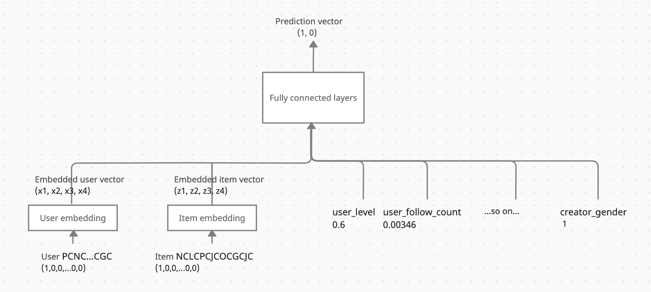
In the training sample, we can see the userId converted to a vector (with a length of the number of users and one indicating which user) in the model. This is the input to the user embedding layer, which converts it into a vector of length 4 (user embedding). A similar process happens with the Items also.
The scaled user and item features directly input the fully connected layers. The input for the fully connected layers is the concatenation of the user embeddings, item embeddings and user and item features.
A sigmoid function is applied at the output layer to obtain the most probable class. In the example, the most probable class is 0.
import torch.nn as nn
# !pip install pytorch_lightning
import pytorch_lightning as pl
from torch.utils.data import DataLoader

class NCF(pl.LightningModule):
    #  Neural Collaborative Filtering (NCF) Ref: https://towardsdatascience.com/deep-learning-based-recommender-systems-3d120201db7e

    def __init__(self, num_users, num_items, users, items, lables, con_var_list):
        super().__init__()
        self.user_embedding = nn.Embedding(num_embeddings=num_users, embedding_dim=4)
        self.item_embedding = nn.Embedding(num_embeddings=num_items, embedding_dim=4)
        self.fc1 = nn.Linear(in_features=8+len(cont_vars), out_features=32)
        self.fc2 = nn.Linear(in_features=32, out_features=16)
        self.output = nn.Linear(in_features=16, out_features=1)
        self.users = users
        self.items = items
        self.lables = lables
        self.con_var_list = con_var_list

    def forward(self, user_input, item_input, con_var_input):

        # Pass through embedding layers
        user_embedded = self.user_embedding(user_input)
        item_embedded = self.item_embedding(item_input)

        # Concat the two embedding layers
        vector = torch.cat([user_embedded, item_embedded, con_var_input], dim=-1)

        # Pass through dense layer
        vector = nn.ReLU()(self.fc1(vector))
        vector = nn.ReLU()(self.fc2(vector))

        # Output layer
        pred = nn.Sigmoid()(self.output(vector))

        return pred

    def training_step(self, batch, batch_idx):
        user_input, item_input, labels, con_var_list = batch
        predicted_labels = self(user_input, item_input, con_var_list)
        loss = nn.BCELoss()(predicted_labels, labels.view(-1, 1).float())
        return loss

    def configure_optimizers(self):
        return torch.optim.Adam(self.parameters())

    def train_dataloader(self):
        return DataLoader(NetEaseTrainDataset(self.users, self.items, self.lables, self.con_var_list),
                          batch_size=512, num_workers=4)
This model is trained for fifty epochs.
num_users = len(selected_users)
num_items = len(selected_mlogs)

model = NCF(num_users, num_items, users, items, lables, con_var_list)

trainer = pl.Trainer(max_epochs=50, logger=False)

trainer.fit(model)
INFO:pytorch_lightning.utilities.rank_zero:GPU available: False, used: False
INFO:pytorch_lightning.utilities.rank_zero:TPU available: False, using: 0 TPU cores
INFO:pytorch_lightning.utilities.rank_zero:IPU available: False, using: 0 IPUs
INFO:pytorch_lightning.utilities.rank_zero:HPU available: False, using: 0 HPUs
INFO:pytorch_lightning.callbacks.model_summary:
  | Name           | Type      | Params
---------------------------------------------
0 | user_embedding | Embedding | 2.9 K
1 | item_embedding | Embedding | 48.1 K
2 | fc1            | Linear    | 640
3 | fc2            | Linear    | 528
4 | output         | Linear    | 17
---------------------------------------------
52.2 K    Trainable params
0         Non-trainable params
52.2 K    Total params
0.209     Total estimated model params size (MB)


Training: 0it [00:00, ?it/s]


INFO:pytorch_lightning.utilities.rank_zero:`Trainer.fit` stopped: `max_epochs=50` reached.
trainer.save_checkpoint("final_model.ckpt")
Evaluating the model
Running the model on the test data, we get an accuracy of 74%.
# need to evaluate the model
test_data = test_data[test_data.userId.isin(selected_users)]
test_data = test_data[test_data.mlogId.isin(selected_mlogs)]
test_data = test_data.reset_index()

users_test, items_test, lables_test = [], [], []
for i in range(len(test_data)):
    users_test.append(users_dict[test_data.userId[i]])
    items_test.append(items_dict[test_data.mlogId[i]])
    lables_test.append(test_data.isClick[i])
con_var_list_test = list(test_data[cont_vars].astype(float).values)
The probability of clicking on the card for the top 20 user specific cards is shown:
# Calculating the probability in the test data
test_data['pred_prob'] = np.squeeze(model(torch.tensor(users_test), torch.tensor(items_test), torch.tensor(con_var_list_test).float()).detach().numpy())
test_data[['isClick', 'pred_prob']].sort_values(['isClick','pred_prob'], ascending=False)[0:20]
| isClick | pred_prob | |
|---|---|---|
| 176772 | 1 | 0.998197 |
| 176774 | 1 | 0.998197 |
| 176794 | 1 | 0.998197 |
| 176780 | 1 | 0.998196 |
| 176773 | 1 | 0.998196 |
| 176778 | 1 | 0.998196 |
| 176787 | 1 | 0.998196 |
| 176783 | 1 | 0.998196 |
| 176786 | 1 | 0.998196 |
| 176767 | 1 | 0.998195 |
| 176784 | 1 | 0.998195 |
| 176785 | 1 | 0.998195 |
| 176791 | 1 | 0.998195 |
| 176788 | 1 | 0.998195 |
| 176775 | 1 | 0.998195 |
| 176782 | 1 | 0.998195 |
| 176766 | 1 | 0.998195 |
| 176776 | 1 | 0.998195 |
| 176781 | 1 | 0.998195 |
| 176790 | 1 | 0.998195 |
As the data is unbalanced, we want to find the optimal probability cutoff for showing a card to a user. We identified the point where a weighted true positivity rate is high, and the weighted false positivity rate is low. The weight indicates the importance given to the positive class.
from sklearn.metrics import roc_curve, auc
import pylab as pl
fpr, tpr, thresholds =roc_curve(test_data.isClick, test_data.pred_prob)
roc_auc = auc(fpr, tpr)
print("Area under the ROC curve : %f" % roc_auc)

####################################
# The optimal cut off would be where tpr is high and fpr is low
# tpr - (1-fpr) is zero or near to zero is the optimal cut off point
####################################
i = np.arange(len(tpr)) # index for df
roc = pd.DataFrame({'fpr' : pd.Series(fpr, index=i),'tpr' : pd.Series(tpr, index = i), '1-fpr' : pd.Series(1-fpr, index = i), 'tf' : pd.Series(tpr - (1-fpr), index = i), 'thresholds' : pd.Series(thresholds, index = i)})
roc.iloc[(roc.tf-0).abs().argsort()[:1]]

# Plot tpr vs 1-fpr
fig, ax = pl.subplots()
pl.plot(roc['tpr'])
pl.plot(roc['1-fpr'], color = 'red')
pl.xlabel('1-False Positive Rate')
pl.ylabel('True Positive Rate')
pl.title('Receiver operating characteristic')
ax.set_xticklabels([])
pl.show()
Area under the ROC curve : 0.552476

cutoff_weight = 3/4
def Find_Optimal_Cutoff(target, predicted):
    # reference https://stackoverflow.com/a/32482924
    fpr, tpr, threshold = roc_curve(target, predicted)
    i = np.arange(len(tpr))
    roc = pd.DataFrame({'tf' : pd.Series((cutoff_weight)*tpr-(1-cutoff_weight)*(1-fpr), index=i), 'threshold' : pd.Series(threshold, index=i)})
    roc_t = roc.iloc[(roc.tf-0).abs().argsort()[:1]]

    return list(roc_t['threshold'])

# Find optimal probability threshold
threshold = Find_Optimal_Cutoff(test_data.isClick, test_data.pred_prob)
print(threshold)
[0.17772053182125092]
The accuracy metrics on the test data are:
from sklearn.metrics import classification_report, confusion_matrix
print(classification_report(test_data.isClick, test_data.pred_prob>0.17))
# confusion_matrix(test_data.isClick, test_data.pred_prob>0.17)
              precision    recall  f1-score   support

           0       0.92      0.79      0.85    220506
           1       0.11      0.28      0.15     20327

    accuracy                           0.74    240833
   macro avg       0.51      0.53      0.50    240833
weighted avg       0.85      0.74      0.79    240833
The alternate way of evaluating the model is by using the Hit Ratio. The user does not need to interact with every single item in the list of recommendations but needs to interact with at least one from all the cards shown. We will consider a user to be "hit" if the user clicks at least one item from the top ten that the user is recommended.
test_data['ranking'] = test_data.groupby('userId').pred_prob.rank(ascending=False)
test_data[test_data.ranking<10].groupby('userId').pred_prob.max().reset_index().pred_prob.mean()
0.42861176
The Hit ratio at 10 is 42.8% (from a 9% hit rate without the recommendation system).
Parts of this work was first used as assignment by Harsha A, Vaibhav D, Akhtar P and Rada G as part of Advanced Machine Learning module at Imperial College London