Understanding Embeddings¶

Embeddings convert text into numbers that a model can compare and reason with. A word, sentence, or paragraph becomes a dense vector, which is a list of values. During training, the model learns which terms appear in similar contexts. Terms with similar use patterns end up closer in vector space. That is why embeddings capture meaning better than plain string matching.

Setting up the Environment¶

We start by importing the libraries and creating an OpenAI client for embedding generation.

from openai import OpenAI
import pandas as pd
import numpy as np
import matplotlib.pyplot as plt
import seaborn as sns
from sklearn.decomposition import PCA
from sklearn.metrics.pairwise import cosine_similarity
from scipy.spatial.distance import cosine
import os

# Replace with your actual API key
client = OpenAI(api_key=os.getenv("OPENAI_API_KEY"))

Generating Embeddings¶

In this section, we generate embeddings for a small group of related words. Modern embedding models use high-dimensional vectors to capture semantic detail. For example, the text-embedding-3-small model returns 1536 values for each input.

words = [
    "king", "queen", "prince", "princess",
    "man", "woman", "boy", "girl",
    "father", "mother",
    "brother", "sister"
]

response = client.embeddings.create(
    model='text-embedding-3-small',
    input=words
)

# Create a dictionary mapping words to their embedding vectors
vectors = {word: item.embedding for word, item in zip(words, response.data)}
embeddings_list = list(vectors.values())

print(f"Vector dimensions for '{words[0]}': {len(embeddings_list[0])}")

Vector dimensions for 'king': 1536

Visualising Dimensions with PCA¶

You can think of each embedding dimension as one learned feature. Since a 1536-dimensional vector cannot be plotted directly, we use Principal Component Analysis (PCA) to project it into two dimensions. This view helps us inspect relative word positions.

pca = PCA(n_components=2)
embedding_2d = pca.fit_transform(embeddings_list)

df = pd.DataFrame(embedding_2d, columns=['PC1', 'PC2'])
df['Word'] = words

plt.figure(figsize=(8, 6))
for i in range(len(df)):
    plt.scatter(df.iloc[i]['PC1'], df.iloc[i]['PC2'], s=100)
    plt.annotate(df.iloc[i]['Word'], (df.iloc[i]['PC1'], df.iloc[i]['PC2']))

plt.title('Word Embeddings Visualised using PCA')
plt.grid(True)
plt.show()

png

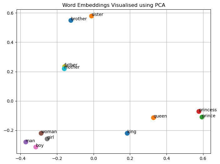
Royal terms appear close to each other, and family pairs such as father-mother and brother-sister also group in nearby regions.

Measuring Similarity¶

To compare semantic closeness, we use cosine similarity. It measures the angle between vectors. A value near 1 means strong alignment, while a value near 0 means weak relation.

\[\cos(\theta)=\frac{\mathbf{A}\cdot\mathbf{B}}{\|\mathbf{A}\|\|\mathbf{B}\|}\]

A heatmap gives a compact view of these pairwise relationships.

import matplotlib.colors as mcolors

# Define the custom colours for each band
colours = [
    'white',     # 0% - 50%
    '#C8E6C9',   # 50% - 60% (light green)
    '#81C784',   # 60% - 70% (green)
    '#4CAF50',   # 70% - 80% (dark green)
    '#2E7D32',   # 80% - 90% (darker green)
    '#1B5E20'    # 90% - 100% (super dark green)
]

# Create the colormap
custom_cmap = mcolors.ListedColormap(colours)

# Define the boundaries corresponding to your percentages
bounds = [0.0, 0.5, 0.6, 0.7, 0.8, 0.9, 1.0]
norm = mcolors.BoundaryNorm(bounds, custom_cmap.N)

similarity_matrix = cosine_similarity(embeddings_list)
similarity_df = pd.DataFrame(similarity_matrix, index=words, columns=words)

plt.figure(figsize=(8, 6))

# Apply the custom colormap and normalisation
# vmin and vmax ensure the scale maps strictly from 0 to 1
sns.heatmap(
    similarity_df, 
    annot=True, 
    cmap=custom_cmap, 
    norm=norm, 
    vmin=0, 
    vmax=1, 
    cbar_kws={'ticks': bounds}
)

plt.title('Cosine Similarity Heatmap')
plt.show()

png

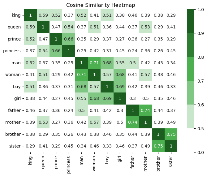
Darker green cells indicate stronger similarity. In this run, pairs like father-mother and brother-sister are among the closest pairs.

Projecting Words onto Conceptual Axes¶

PCA finds global variance directions automatically. We can also define manual semantic directions to test specific concepts.

To build an axis, we subtract one anchor vector from another. Here, we create a "Gender" axis and a "Royalty" axis, then project each word onto both. This shows how one embedding can encode more than one attribute.

# Convert lists to numpy arrays for vector arithmetic
vec_man = np.array(vectors['man'])
vec_woman = np.array(vectors['woman'])
vec_king = np.array(vectors['king'])

# Define direction vectors for the semantic axes
gender_axis = vec_woman - vec_man
royalty_axis = vec_king - vec_man

royalty_scores = []
gender_scores = []

for word in words:
    # 1 - cosine distance gives the cosine similarity
    royal = 1 - cosine(vectors[word], royalty_axis)
    gender = 1 - cosine(vectors[word], gender_axis)

    royalty_scores.append(royal)
    gender_scores.append(gender)

plt.figure(figsize=(10, 8))

for i, word in enumerate(words):
    plt.scatter(royalty_scores[i], gender_scores[i], s=120)
    plt.text(royalty_scores[i] + 0.005, gender_scores[i] + 0.005, word)

plt.axhline(0, color='grey', linestyle='--')
plt.axvline(0, color='grey', linestyle='--')

plt.xlabel("Royalty")
plt.ylabel("Male ↔ Female")
plt.title("Concept Directions in Embedding Space")
plt.grid(True)
plt.show()

png

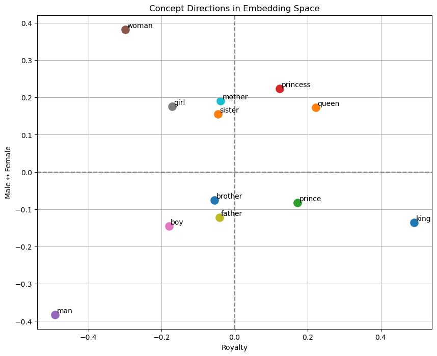
King and prince appear in the male-royalty region, while queen and princess appear in the female-royalty region. Non-royal terms spread across the space based on gender direction.

Moving from Word to Sentence Embeddings¶

In early NLP systems such as Word2Vec and GloVe, each word had one fixed vector. A sentence vector was often created by averaging word vectors. This lost word order and context. For example, "dog bites man" and "man bites dog" could look similar after averaging.

Modern embedding pipelines address this with subword tokenisation and Transformer attention:

Subword tokenisation: Methods such as BPE or WordPiece split unknown words into known fragments, which improves coverage.
Contextual token representation: Self-attention updates each token using the full sequence context. So "bank" in "river bank" and "investment bank" maps differently.
Pooling: The model compresses token-level outputs into one vector, often through a classification token or mean pooling.
Contrastive learning: Embedding models are trained to pull related sentences closer and push unrelated ones apart.

Cosine Similarity for Retrieval¶

In high-dimensional spaces, vector magnitude can vary with writing style or sentence length. Cosine similarity focuses on direction, which is often better for retrieval than raw Euclidean distance:

\[\text{Cosine Similarity}(\mathbf{u}, \mathbf{v}) = \frac{\mathbf{u} \cdot \mathbf{v}}{\Vert{}\mathbf{u}\Vert{} \Vert{}\mathbf{v}\Vert{}} = \frac{\sum_{i=1}^{n} u_i v_i}{\sqrt{\sum_{i=1}^{n} u_i^2} \sqrt{\sum_{i=1}^{n} v_i^2}}\]

When vectors are normalised to unit length (\(\Vert{}\mathbf{u}\Vert{} = 1\)), cosine similarity reduces to the dot product \(\mathbf{u} \cdot \mathbf{v}\).

Retrieving the Top 3 Sentences¶

The final example embeds a 10-sentence knowledge base, embeds one query, and retrieves the top three matches.

import numpy as np
import pandas as pd
from openai import OpenAI
from sklearn.metrics.pairwise import cosine_similarity

# 1. Define our knowledge base (10 sentences across different topics)
documents = [
    "The Reserve Bank of India manages the monetary policy and currency supply.",
    "Photosynthesis allows green plants to convert sunlight into chemical energy.",
    "Supervised learning algorithms require labelled datasets for model training.",
    "Bengaluru is widely known as the primary technology hub of India.",
    "A retrieval-augmented generation pipeline extracts context from a vector database.",
    "The Indian cricket team won the ICC Champions Trophy tournament.",
    "Convolutional neural networks excel at spatial feature extraction in images.",
    "Chlorophyll pigments absorb blue and red light while reflecting green wavelengths.",
    "Vector embeddings map distinct concepts into continuous mathematical spaces.",
    "Regular physical exercise improves cardiovascular health and stamina."
]

# 2. Define the query prompt
query = "How do machine learning models learn from data representations?"

# 3. Generate embeddings for both the corpus and the query
# We bundle all texts into a single API call for efficiency
all_texts = [query] + documents

response = client.embeddings.create(
    model="text-embedding-3-small",
    input=all_texts
)

# Extract embedding vectors
all_embeddings = [item.embedding for item in response.data]
query_vector = np.array(all_embeddings[0]).reshape(1, -1)
doc_vectors = np.array(all_embeddings[1:])

# 4. Calculate Cosine Similarity
similarity_scores = cosine_similarity(query_vector, doc_vectors)[0]

# 5. Rank and retrieve the top 3 matches
top_k = 3
top_indices = np.argsort(similarity_scores)[::-1][:top_k]

# Display results
print(f"Query: \"{query}\"\n")
print("Top Relevant Documents:")
print("-" * 60)

for rank, idx in enumerate(top_indices, start=1):
    score = similarity_scores[idx]
    sentence = documents[idx]
    print(f"Rank {rank} (Score: {score:.4f}):")
    print(f"  {sentence}\n")

Query: "How do machine learning models learn from data representations?"

Top Relevant Documents:
------------------------------------------------------------
Rank 1 (Score: 0.4189):
  Supervised learning algorithms require labelled datasets for model training.

Rank 2 (Score: 0.3885):
  Vector embeddings map distinct concepts into continuous mathematical spaces.

Rank 3 (Score: 0.3064):
  Convolutional neural networks excel at spatial feature extraction in images.