Streaming machine learning
Author: Achyuthuni Sri Harsha
originally published at R2DL Library on 17th April 2021.
Batch learning: In batch machine learning, we use one dataset to train a model, and we deploy the model to predict on new data. This assumes that the dataset in which the model is trained is a proper representative sample of the population. This model is assumed as a static object. In order to learn from new data, the model has to be re-trained from scratch. This is the most common form of deploying models.
Online learning: Some machine learning models that we know can be modified to learn on a single data point (row). When we can learn from a single data point, we can learn incrementally from new data points. Data is considered as a stream. Once the model is trained, we need not store the historic training set. The model is also more up to date. If the data's distribution happens over time, the model will be able to handle it (drift)[1].
Where can we use them?
They are most useful in scenarios where new data and patterns are constantly arriving. Example:
1. Spam filtering
2. Recommendation engines (news feed predictions)
3. Financial transactions
4. Low compute power (only one data point exists in memory as we train using one data point only)
Issues
1. New and not a lot of experience
2. Very few tools and packages
3. All algorithms do not have an online version. Kernel SVM's are impossible to fit on a streaming dataset. Likewise, CART and ID3 decision trees can’t be trained online. However, lesser-known online approximations exist, such as random Fourier features for SVM's and Hoeffding trees for decision trees.
4. Slower than batch learning to reach steady state in real life (It is computationally faster by more than an order of magnitude)
5. Do not guarantee that models learnt are similar to the ones obtained in batch mode(some models). Some models do not guarantee of achieving steady state.
6. Overfitting
Similarities
We have the same limitations of machine learning, such as:
1. We need to do proper preprocessing
2. We need to do feature engineering as usual
3. The concepts of ensembles, feature extraction, feature selection, imbalanced classes, multiclass etc are same
Preprocessing steps
How do we preprocess data when we are streaming? How do we impute the null values by mean if we do not have complete data? How do we identify outliers when working on one row at a time? How can we do one-hot encoding when we don't know what classes are present overall? The package river is a handy package for online learning. It has a lot of pre-defined preprocessing functions. Let us look at some of them:
from river import preprocessing
dir(preprocessing)[0:12]
['AdaptiveStandardScaler',
 'Binarizer',
 'FeatureHasher',
 'LDA',
 'MaxAbsScaler',
 'MinMaxScaler',
 'Normalizer',
 'OneHotEncoder',
 'PreviousImputer',
 'RobustScaler',
 'StandardScaler',
 'StatImputer']
There are six functions for scaling and normalizing data. They are:
1. AdaptiveStandardScalar
2. MaxAbsScalar
3. MinMaxScalar
4. Normalizer
5. RobustScalar
6. StandardScaler
For example, let us look at the documentation for Standard Scaler It scales the data to have zero mean and unit variance.
Under the hood, a running mean and a running variance are maintained. The scaling is slightly different from when scaling the data in batch because the exact means and variances are not known in advance. However, this doesn't have a detrimental impact on performance in the long run.
Let us look at an example:
import numpy as np
import matplotlib.pyplot as plt
import pandas as pd
import random

random.seed(1995)

from sklearn.datasets import load_iris
iris = load_iris()
data1 = pd.DataFrame(data= np.c_[iris['data'], iris['target']],
                     columns= iris['feature_names'] + ['target'])
data1 = data1.query('target < 2').sample(frac=1)
def data_feed(df_datafeed):
    # Generator function to give the next candidate
    for _ctr in range(len(df_datafeed)):
        yield df_datafeed.iloc[_ctr]
from river import compose
from river import linear_model
from river import preprocessing

preprocessing_model = compose.Pipeline(
            preprocessing.StandardScaler(),
            linear_model.LogisticRegression())


data_stream = data_feed(data1.loc[:,data1.columns != 'target'])
for n in range(10):
    data_point = next(data_stream).to_frame().transpose()

    transformed_data = preprocessing_model.transform_one(data_point.iloc[0,:])

    print('------------------------')
    print(data_point)
    print(transformed_data)
------------------------
    sepal length (cm)  sepal width (cm)  petal length (cm)  petal width (cm)
67                5.8               2.7                4.1               1.0
{'sepal length (cm)': 0.0, 'sepal width (cm)': 0.0, 'petal length (cm)': 0.0, 'petal width (cm)': 0.0}
------------------------
    sepal length (cm)  sepal width (cm)  petal length (cm)  petal width (cm)
96                5.7               2.9                4.2               1.3
{'sepal length (cm)': -1.0, 'sepal width (cm)': 1.000000000000001, 'petal length (cm)': 0.9999999999999956, 'petal width (cm)': 1.0000000000000004}
------------------------
    sepal length (cm)  sepal width (cm)  petal length (cm)  petal width (cm)
19                5.1               3.8                1.5               0.3
{'sepal length (cm)': -1.4018260516446994, 'sepal width (cm)': 1.3934660285832352, 'petal length (cm)': -1.4134589797160622, 'petal width (cm)': -1.352447383098741}
------------------------
   sepal length (cm)  sepal width (cm)  petal length (cm)  petal width (cm)
5                5.4               3.9                1.7               0.4
{'sepal length (cm)': -0.36514837167010933, 'sepal width (cm)': 1.0830277015004253, 'petal length (cm)': -0.9198021534721369, 'petal width (cm)': -0.8427009716003844}
------------------------
    sepal length (cm)  sepal width (cm)  petal length (cm)  petal width (cm)
64                5.6               2.9                3.6               1.3
{'sepal length (cm)': 0.32232918561015234, 'sepal width (cm)': -0.6740938478604231, 'petal length (cm)': 0.49202037860731096, 'petal width (cm)': 1.019130320146575}
------------------------
    sepal length (cm)  sepal width (cm)  petal length (cm)  petal width (cm)
87                6.3               2.3                4.4               1.3
{'sepal length (cm)': 1.7636409634199253, 'sepal width (cm)': -1.3539553245018423, 'petal length (cm)': 0.9642101587457326, 'petal width (cm)': 0.8589556903873334}
------------------------
    sepal length (cm)  sepal width (cm)  petal length (cm)  petal width (cm)
80                5.5               2.4                3.8               1.1
{'sepal length (cm)': -0.37242264987106416, 'sepal width (cm)': -0.9985160994941403, 'petal length (cm)': 0.4205955120960296, 'petal width (cm)': 0.3575992699260759}
------------------------
    sepal length (cm)  sepal width (cm)  petal length (cm)  petal width (cm)
98                5.1               2.5                3.0               1.1
{'sepal length (cm)': -1.259494647504126, 'sepal width (cm)': -0.743358098059264, 'petal length (cm)': -0.27274857904612027, 'petal width (cm)': 0.331861655799986}
------------------------
    sepal length (cm)  sepal width (cm)  petal length (cm)  petal width (cm)
15                5.7               4.4                1.5               0.4
{'sepal length (cm)': 0.3503113654141663, 'sepal width (cm)': 1.8442002991885438, 'petal length (cm)': -1.3918304919158082, 'petal width (cm)': -1.282736189026269}
------------------------
    sepal length (cm)  sepal width (cm)  petal length (cm)  petal width (cm)
23                5.1               3.3                1.7               0.5
{'sepal length (cm)': -1.1921469919530685, 'sepal width (cm)': 0.28047526828011227, 'petal length (cm)': -1.077226017628646, 'petal width (cm)': -0.9305415914315355}
Apart from preprocessing, using river, we can perform
1. Feature extraction/selection
2. Ensembles
3. Storing running statistics
4. Building regression and classification models
5. Time series
6. Anomaly detection
7. Clustering
There are 6 types of machine learning models that we can build using river. They are:
1. Linear based (linear and logistic regression)
2. Tree based (Decision trees, Hoeffding trees)
3. Nearest neighbours based
4. Bayesian models
5. Neural Networks
6. Ensemble based models
7. Others
from river import linear_model, naive_bayes, tree, neural_net, neighbors, expert, ensemble
print('Linear models', dir(linear_model)[0:7])
print('Tree based modles', dir(tree)[0:6])
print('Bayesian models', dir(naive_bayes)[0:4])
print('Specialised models', dir(expert)[0:6])
print('Ensemble mmodels', dir(ensemble)[0:8])
Linear models ['ALMAClassifier', 'LinearRegression', 'LogisticRegression', 'PAClassifier', 'PARegressor', 'Perceptron', 'SoftmaxRegression']
Tree based modles ['ExtremelyFastDecisionTreeClassifier', 'HoeffdingAdaptiveTreeClassifier', 'HoeffdingAdaptiveTreeRegressor', 'HoeffdingTreeClassifier', 'HoeffdingTreeRegressor', 'LabelCombinationHoeffdingTreeClassifier']
Bayesian models ['BernoulliNB', 'ComplementNB', 'GaussianNB', 'MultinomialNB']
Specialised models ['EWARegressor', 'EpsilonGreedyRegressor', 'StackingClassifier', 'SuccessiveHalvingClassifier', 'SuccessiveHalvingRegressor', 'UCBRegressor']
Ensemble mmodels ['ADWINBaggingClassifier', 'AdaBoostClassifier', 'AdaptiveRandomForestClassifier', 'AdaptiveRandomForestRegressor', 'BaggingClassifier', 'BaggingRegressor', 'LeveragingBaggingClassifier', 'SRPClassifier']
Modelling (under the hood)
There are two types of streaming models, those which are entirely streaming and pseudo-online models. Pseudo-online models use a small batch of data to build the models, while completely online models build the models using only one data point.[3]
Pseudo online models
There are many theorems in statistics which can help us to bound the error of a metric between two variables. Hoeffding bound is one such theorem.
"Consider a real-valued random variable r whose range is R (e.g., for a probability the range is one, and for an information gain the range is log c, where c is the number of classes). Suppose we have made n independent observations of this variable, and computed their mean \(\bar r\). The Hoeffding bound states that, with probability 1 − δ, the true mean of the variable is at least \(\bar r − \epsilon\), where \(\epsilon = \sqrt{\frac{R^2ln(\frac{1}{\lambda})}{2n}}\)."
This is useful while creating decision trees. Using hoeffding bound, we can identify which feature should we use to split the tree. We can find if a variable has sufficient gini index (or other metrics) greater (lesser) than other variables with a probability below a cut-off probability and split the tree based on that metric. This can be achieved with very few data points which can be deleted after splitting and creating child nodes. This algorithm is called Hoeffding trees algorithm.
Completely online models
How can we update a model using only one data point? Let us look at Gradient Descent to understand this. In gradient descent, we want to minimise a convex loss function(MSE, regret, etc). As an example, consider the function \(h(x) = \beta_0 + \beta_1 x_1 + \beta_2 x_2 + ..\) (or any convex function). The mean squared error is \(J(\theta) = \frac{1}{2} \sum_{i=1}^{m} (y_{(i)}-h_{\theta}(x_{(i)}))^{2}\). In gradient descent, we find the \(\beta_i\) that minimises \(J(\theta)\).
In batch model, we consider all the data points that exist to identify the optimal solution. In streaming learning, we initialise the \(\beta_i\) as 0 and keep incrementally changing the \(\beta_i\)'s using $$ \beta_{i, t} = \beta_{i, t-1} + \alpha \times \frac{\partial}{\partial \theta_{j}} J(\theta) $$
Steps in updating the model
In online learning, there are 4 steps[3]. For every new data point, we will recursively run the following steps.
For \({\displaystyle t=1,2,...,T}\)
- Learner receives input \({\displaystyle x_{t}}\)
- Learner outputs \({\displaystyle w_{t}}\) from a fixed convex set \({\displaystyle S}\)
- Nature sends back a convex loss function \({\displaystyle v_{t}:S\rightarrow \mathbb {R} }\).
- Learner suffers loss \({\displaystyle v_{t}(w_{t})}\) and updates its model.
Implementation using river
Every online machine learning model has the following basic 5 functions:
dir(linear_model.LogisticRegression)[50:55]
['learn_many',
 'learn_one',
 'predict_many',
 'predict_one',
 'predict_proba_many']
As the name mentions, learn_one and predict_one learn and predict from one data point, learn_many, predict_many and predict_prob_many learn and predict using multiple data points. River is the result of a merger between creme and scikit-multiflow, and the remaining functions in the library follow a similar pattern to the same.
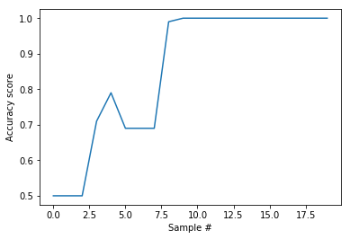
Building a model
Using the same data as above, let us build a sample model using river for streaming.
from river import compose

river_model = compose.Pipeline(
    preprocessing.StandardScaler(),
    tree.HoeffdingTreeClassifier()
)
from sklearn.metrics import accuracy_score

acc_scores = []
cols_x = ['sepal length (cm)', 'sepal width (cm)', 'petal length (cm)', 'petal width (cm)']
def compute_accuracy(data, model, truth_col):
    predict_all = data.apply(lambda row: model.predict_one(row), axis=1)
    acc_scores.append(accuracy_score(np.array(predict_all),data[truth_col]))
    print('Accuracy is ', acc_scores[-1])

data_stream = data_feed(data1)
for n in range(20):
    data_point = next(data_stream)
    print(data_point)
    if(n>1):
        predict_one = river_model.predict_one(data_point[cols_x])
        print('Current_prediction', predict_one, data_point['target'])

    river_model.learn_one(data_point[cols_x],data_point['target'])

    compute_accuracy(data1, river_model, 'target')
    print('------------------------')
sepal length (cm)    5.8
sepal width (cm)     2.7
petal length (cm)    4.1
petal width (cm)     1.0
target               1.0
Name: 67, dtype: float64
Accuracy is  0.5
------------------------
sepal length (cm)    5.7
sepal width (cm)     2.9
petal length (cm)    4.2
petal width (cm)     1.3
target               1.0
Name: 96, dtype: float64
Accuracy is  0.5
------------------------
sepal length (cm)    5.1
sepal width (cm)     3.8
petal length (cm)    1.5
petal width (cm)     0.3
target               0.0
Name: 19, dtype: float64
Current_prediction 1.0 0.0
Accuracy is  0.5
------------------------
sepal length (cm)    5.4
sepal width (cm)     3.9
petal length (cm)    1.7
petal width (cm)     0.4
target               0.0
Name: 5, dtype: float64
Current_prediction 1.0 0.0
Accuracy is  0.71
------------------------
sepal length (cm)    5.6
sepal width (cm)     2.9
petal length (cm)    3.6
petal width (cm)     1.3
target               1.0
Name: 64, dtype: float64
Current_prediction 1.0 1.0
Accuracy is  0.79
------------------------
sepal length (cm)    6.3
sepal width (cm)     2.3
petal length (cm)    4.4
petal width (cm)     1.3
target               1.0
Name: 87, dtype: float64
Current_prediction 1.0 1.0
Accuracy is  0.69
------------------------
sepal length (cm)    5.5
sepal width (cm)     2.4
petal length (cm)    3.8
petal width (cm)     1.1
target               1.0
Name: 80, dtype: float64
Current_prediction 1.0 1.0
Accuracy is  0.69
------------------------
sepal length (cm)    5.1
sepal width (cm)     2.5
petal length (cm)    3.0
petal width (cm)     1.1
target               1.0
Name: 98, dtype: float64
Current_prediction 1.0 1.0
Accuracy is  0.69
------------------------
sepal length (cm)    5.7
sepal width (cm)     4.4
petal length (cm)    1.5
petal width (cm)     0.4
target               0.0
Name: 15, dtype: float64
Current_prediction 1.0 0.0
Accuracy is  0.99
------------------------
sepal length (cm)    5.1
sepal width (cm)     3.3
petal length (cm)    1.7
petal width (cm)     0.5
target               0.0
Name: 23, dtype: float64
Current_prediction 0.0 0.0
Accuracy is  1.0
------------------------
sepal length (cm)    4.8
sepal width (cm)     3.1
petal length (cm)    1.6
petal width (cm)     0.2
target               0.0
Name: 30, dtype: float64
Current_prediction 0.0 0.0
Accuracy is  1.0
------------------------
sepal length (cm)    5.5
sepal width (cm)     2.5
petal length (cm)    4.0
petal width (cm)     1.3
target               1.0
Name: 89, dtype: float64
Current_prediction 1.0 1.0
Accuracy is  1.0
------------------------
sepal length (cm)    4.5
sepal width (cm)     2.3
petal length (cm)    1.3
petal width (cm)     0.3
target               0.0
Name: 41, dtype: float64
Current_prediction 0.0 0.0
Accuracy is  1.0
------------------------
sepal length (cm)    6.1
sepal width (cm)     3.0
petal length (cm)    4.6
petal width (cm)     1.4
target               1.0
Name: 91, dtype: float64
Current_prediction 1.0 1.0
Accuracy is  1.0
------------------------
sepal length (cm)    5.2
sepal width (cm)     3.5
petal length (cm)    1.5
petal width (cm)     0.2
target               0.0
Name: 27, dtype: float64
Current_prediction 0.0 0.0
Accuracy is  1.0
------------------------
sepal length (cm)    7.0
sepal width (cm)     3.2
petal length (cm)    4.7
petal width (cm)     1.4
target               1.0
Name: 50, dtype: float64
Current_prediction 1.0 1.0
Accuracy is  1.0
------------------------
sepal length (cm)    5.5
sepal width (cm)     4.2
petal length (cm)    1.4
petal width (cm)     0.2
target               0.0
Name: 33, dtype: float64
Current_prediction 0.0 0.0
Accuracy is  1.0
------------------------
sepal length (cm)    5.9
sepal width (cm)     3.2
petal length (cm)    4.8
petal width (cm)     1.8
target               1.0
Name: 70, dtype: float64
Current_prediction 1.0 1.0
Accuracy is  1.0
------------------------
sepal length (cm)    6.6
sepal width (cm)     3.0
petal length (cm)    4.4
petal width (cm)     1.4
target               1.0
Name: 75, dtype: float64
Current_prediction 1.0 1.0
Accuracy is  1.0
------------------------
sepal length (cm)    4.4
sepal width (cm)     3.0
petal length (cm)    1.3
petal width (cm)     0.2
target               0.0
Name: 38, dtype: float64
Current_prediction 0.0 0.0
Accuracy is  1.0
------------------------
import matplotlib.pyplot as plt
%matplotlib inline
plt.plot(acc_scores)
plt.ylabel('Accuracy score')
plt.xlabel('Sample #')
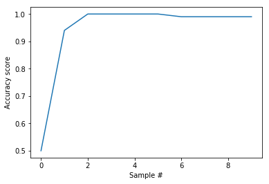
river_model2 = compose.Pipeline(
    preprocessing.StandardScaler(),
    linear_model.LogisticRegression()
)

acc_scores1 = []
def compute_accuracy(data, model, truth_col):
    predict_all = data.apply(lambda row: model.predict_one(row), axis=1)
    acc_scores1.append(accuracy_score(np.array(predict_all),data[truth_col]))
    print('Accuracy is ', acc_scores1[-1])

data_stream = data_feed(data1)
for n in range(10):
    data_point = next(data_stream)
    print(data_point)
    if(n>1):
        predict_one = river_model2.predict_one(data_point[cols_x])
        print('Current_prediction', predict_one, data_point['target'])

    river_model2.learn_one(data_point[cols_x],data_point['target'])

    compute_accuracy(data1, river_model2, 'target')
    print('------------------------')
sepal length (cm)    5.8
sepal width (cm)     2.7
petal length (cm)    4.1
petal width (cm)     1.0
target               1.0
Name: 67, dtype: float64
Accuracy is  0.5
------------------------
sepal length (cm)    5.7
sepal width (cm)     2.9
petal length (cm)    4.2
petal width (cm)     1.3
target               1.0
Name: 96, dtype: float64
Accuracy is  0.94
------------------------
sepal length (cm)    5.1
sepal width (cm)     3.8
petal length (cm)    1.5
petal width (cm)     0.3
target               0.0
Name: 19, dtype: float64
Current_prediction False 0.0
Accuracy is  1.0
------------------------
sepal length (cm)    5.4
sepal width (cm)     3.9
petal length (cm)    1.7
petal width (cm)     0.4
target               0.0
Name: 5, dtype: float64
Current_prediction False 0.0
Accuracy is  1.0
------------------------
sepal length (cm)    5.6
sepal width (cm)     2.9
petal length (cm)    3.6
petal width (cm)     1.3
target               1.0
Name: 64, dtype: float64
Current_prediction True 1.0
Accuracy is  1.0
------------------------
sepal length (cm)    6.3
sepal width (cm)     2.3
petal length (cm)    4.4
petal width (cm)     1.3
target               1.0
Name: 87, dtype: float64
Current_prediction True 1.0
Accuracy is  1.0
------------------------
sepal length (cm)    5.5
sepal width (cm)     2.4
petal length (cm)    3.8
petal width (cm)     1.1
target               1.0
Name: 80, dtype: float64
Current_prediction True 1.0
Accuracy is  0.99
------------------------
sepal length (cm)    5.1
sepal width (cm)     2.5
petal length (cm)    3.0
petal width (cm)     1.1
target               1.0
Name: 98, dtype: float64
Current_prediction True 1.0
Accuracy is  0.99
------------------------
sepal length (cm)    5.7
sepal width (cm)     4.4
petal length (cm)    1.5
petal width (cm)     0.4
target               0.0
Name: 15, dtype: float64
Current_prediction False 0.0
Accuracy is  0.99
------------------------
sepal length (cm)    5.1
sepal width (cm)     3.3
petal length (cm)    1.7
petal width (cm)     0.5
target               0.0
Name: 23, dtype: float64
Current_prediction False 0.0
Accuracy is  0.99
------------------------
import matplotlib.pyplot as plt
%matplotlib inline
plt.plot(acc_scores1)
plt.ylabel('Accuracy score')
plt.xlabel('Sample #')
First published on Rolls-Royce data science blogs by Harsha Achyuthuni.
References
- Introductory material: https://towardsdatascience.com/machine-learning-for-streaming-data-with-creme-dacf5fb469df
- Hoeffding Trees: https://homes.cs.washington.edu/~pedrod/papers/kdd00.pdf
- Modelling under the hood: https://en.wikipedia.org/wiki/Online_machine_learning
- River Git: https://github.com/online-ml/river
- River installation steps: https://riverml.xyz/dev/getting-started/installation/
- River documentation: https://riverml.xyz/dev/api/overview/
- Batch decision trees: blog