Tensorflow and Keras

Introduction¶

In the first two blogs, we covered perceptron and backpropagation. We have also worked on the absenteeism categorization problem in feature engineering and machine learning. In this blog, we will build a basic neural network with Tensorflow and Keras to predict who will be absent in the future.

TensorFlow and Keras¶

TensorFlow is a robust, open-source library for numerical computation and large-scale machine learning. Keras, on the other hand, is a high-level neural network API built on top of TensorFlow. Keras helps in building, training, executing, and evaluating all kinds of neural networks.

Data¶

Organizations face a significant challenge in motivating their employees. This is the continuation of a blog series in which we used several feature engineering strategies to create a comprehensive dataset and then predicted who would be absent using machine learning and Scikit-Learn. In this blog, we will use this information to predict employee absenteeism. The purpose is to identify those who are likely to be absent in the near future.

As a first step, load and examine the data.

import pandas as pd
%matplotlib inline
import matplotlib.pyplot as plt
import random
import numpy as np
np.random.seed(42)
df = pd.read_csv('/content/gdrive/MyDrive/data_after_feature_engg.csv')
df

	Unnamed: 0	employee	date	last_likes	last_dislikes	feedbackType	likes_till_date	dislikes_till_date	last_2_likes	last_2_dislikes	...	employee_joined_after_jun17	countdown_to_last_day	reason	on_leave	no_leaves_till_date	last_2_days_leaves	previous_day_leave	weekday	month	week
0	23729	17r	2018-05-29	0.0	0.0	0	0.0	0.0	0.0	0.0	...	1.0	999	NaN	0.0	0.0	0.0	0.0	Tuesday	May	1
1	23730	17r	2018-05-30	0.0	0.0	0	0.0	0.0	0.0	0.0	...	1.0	999	NaN	0.0	0.0	0.0	0.0	Wednesday	May	2
2	23731	17r	2018-05-31	0.0	0.0	0	0.0	0.0	0.0	0.0	...	1.0	999	NaN	0.0	0.0	0.0	0.0	Thursday	May	3
3	23732	17r	2018-06-01	0.0	0.0	0	0.0	0.0	0.0	0.0	...	1.0	999	NaN	0.0	0.0	0.0	0.0	Friday	Jun	1
4	23733	17r	2018-06-02	0.0	0.0	0	0.0	0.0	0.0	0.0	...	1.0	999	NaN	0.0	0.0	0.0	0.0	Saturday	Jun	2
...	...	...	...	...	...	...	...	...	...	...	...	...	...	...	...	...	...	...	...	...	...
33446	32232	zGB	2019-03-07	24.0	8.0	OTHER	24.0	8.0	24.0	8.0	...	0.0	999	NaN	0.0	0.0	0.0	0.0	Thursday	Mar	0
33447	32233	zGB	2019-03-08	24.0	8.0	OTHER	24.0	8.0	24.0	8.0	...	0.0	999	NaN	0.0	0.0	0.0	0.0	Friday	Mar	1
33448	32234	zGB	2019-03-09	24.0	8.0	OTHER	24.0	8.0	24.0	8.0	...	0.0	999	NaN	0.0	0.0	0.0	0.0	Saturday	Mar	2
33449	32235	zGB	2019-03-10	24.0	8.0	OTHER	24.0	8.0	24.0	8.0	...	0.0	999	NaN	0.0	0.0	0.0	0.0	Sunday	Mar	3
33450	32236	zGB	2019-03-11	24.0	8.0	OTHER	24.0	8.0	24.0	8.0	...	0.0	999	NaN	0.0	0.0	0.0	0.0	Monday	Mar	4

33451 rows × 31 columns

In the previous blog, we created the key features required for this binary classification task. All of these variables are listed in indep_vars.

from sklearn.model_selection import train_test_split, GridSearchCV
indep_vars = ['last_likes', 'last_dislikes', 'feedbackType',
     'likes_till_date', 'dislikes_till_date', 'last_2_likes', 'last_2_dislikes',
     'days_since_last_comment', 'last_vote', 'timezone', 'stillExists',
       'no_of_days_since_first_vote', 'no_of_votes_till_date',
       'perc_days_voted', 'avg_vote_till_date', 'avg_vote', 'last_2_votes_avg',
       'days_since_last_vote', 'employee_joined_after_jun17', 'countdown_to_last_day',
        'no_leaves_till_date', 'weekday', 'month']
data_targets = df['on_leave'].astype('int')
data_features = pd.get_dummies(df[indep_vars], prefix = "_", drop_first= True)

x_train, x_test, y_train, y_test = train_test_split(data_features, data_targets, test_size=.30, random_state=35, \
                                                    stratify=data_targets)

We then scale every independent variable. This promotes faster convergence, reduces the vanishing gradient problem, and increases stability. We will look into these concerns later.

from sklearn.preprocessing import StandardScaler
sc = StandardScaler()
x_train = sc.fit_transform(x_train)
x_test = sc.transform(x_test)

input_length = len(x_train[0])

Sequential API¶

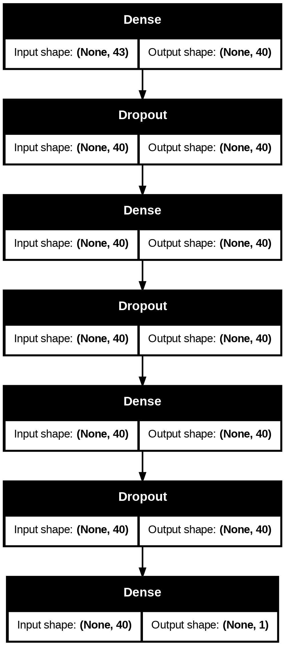
Keras provides two basic approaches: a sequential model API and a functional model API. The sequential model API works well for the majority of basic neural networks. Let us build a simple neural network with one input layer, three hidden layers, and one output layer. The hidden layers use the ReLU activation function, whereas the output layer uses the sigmoid activation function.

import tensorflow as tf
from tensorflow import keras
from keras.models import Sequential
from keras.layers import Dense, Dropout, InputLayer
model = Sequential([
    InputLayer(input_shape = [input_length], name='Input_layer'),
    Dense(40, activation="relu", name = 'Hidden_layer_1'),
    Dropout(rate=0.1, name='Dropout_layer_1'),
    Dense(40, activation="relu", name = 'Hidden_layer_2'),
    Dropout(rate=0.1, name='Dropout_layer_2'),
    Dense(40, activation="relu", name = 'Hidden_layer_3'),
    Dropout(rate=0.1, name='Dropout_layer_3'),
    Dense(1, activation="sigmoid", name = 'Output_layer')
])

The hidden layers each have 40 neurons while the output layer has 1 neuron. The output layer represents the likelihood of being absent.

Number of parameters¶

In this simple network, the number of parameters in each layer is the same as the number of connections. In any layer, $$ Number\,of\,connections = (input_length+1)\times(output_length) $$ $Number\,of\,input\,neurons = input\_neurons+bias\_neuron = input\_length+1$
1. Hidden_layer_1: (43+1)x(40) = 1760
2. Hidden_layer_2: (40+1)x(40) = 1640
3. Hidden_layer_3: (40+1)x(40) = 1640
4. Output_layer: (40+1)x(1) = 41

model.summary()

Model: "sequential"

┏━━━━━━━━━━━━━━━━━━━━━━━━━━━━━━━━━━━━━━┳━━━━━━━━━━━━━━━━━━━━━━━━━━━━━┳━━━━━━━━━━━━━━━━━┓
┃ Layer (type)                         ┃ Output Shape                ┃         Param # ┃
┡━━━━━━━━━━━━━━━━━━━━━━━━━━━━━━━━━━━━━━╇━━━━━━━━━━━━━━━━━━━━━━━━━━━━━╇━━━━━━━━━━━━━━━━━┩
│ Hidden_layer_1 (Dense)               │ (None, 40)                  │           1,760 │
├──────────────────────────────────────┼─────────────────────────────┼─────────────────┤
│ Dropout_layer_1 (Dropout)            │ (None, 40)                  │               0 │
├──────────────────────────────────────┼─────────────────────────────┼─────────────────┤
│ Hidden_layer_2 (Dense)               │ (None, 40)                  │           1,640 │
├──────────────────────────────────────┼─────────────────────────────┼─────────────────┤
│ Dropout_layer_2 (Dropout)            │ (None, 40)                  │               0 │
├──────────────────────────────────────┼─────────────────────────────┼─────────────────┤
│ Hidden_layer_3 (Dense)               │ (None, 40)                  │           1,640 │
├──────────────────────────────────────┼─────────────────────────────┼─────────────────┤
│ Dropout_layer_3 (Dropout)            │ (None, 40)                  │               0 │
├──────────────────────────────────────┼─────────────────────────────┼─────────────────┤
│ Output_layer (Dense)                 │ (None, 1)                   │              41 │
└──────────────────────────────────────┴─────────────────────────────┴─────────────────┘

 Total params: 5,081 (19.85 KB)

 Trainable params: 5,081 (19.85 KB)

 Non-trainable params: 0 (0.00 B)

Dense layer¶

A dense layer is a fully connected layer of neurons that receives input from every neuron in the previous layer.

Dropout¶

Dropout is the most popular form of regularization technique in which certain nodes are ignored at random during training. Adding dropout layer improves accuracy by 1-2% on average. In a dropout layer, at any training step, every neuron in the previous layer has a probability (equal to the rate) of dropping out. This dropped-out node may be active in the following step/epoch. Dropouts are said to improve the resilience of the network.

accuracy_metrics = [
    "accuracy", "Recall", "Precision",
    keras.metrics.FalseNegatives(name="fn"),
    keras.metrics.FalsePositives(name="fp"),
    keras.metrics.TrueNegatives(name="tn"),
    keras.metrics.TruePositives(name="tp")
]
model.compile(loss="binary_crossentropy",  optimizer="sgd",  metrics=accuracy_metrics)

x_train = np.asarray(x_train).astype('float32')
x_test = np.asarray(x_test).astype('float32')
y_train = np.array(y_train)
y_test = np.array(y_test)

There is a huge imbalance in the data. To balance the data, we are giving weights inversely proportional to the class frequency.

class_weights = {0:len(y_train)/sum(y_train==0), 1:len(y_train)/sum(y_train==1)}
class_weights

{0: 1.0510368973875572, 1: 20.593667546174142}

Fitting the model for 100 epochs

history = model.fit(x_train, y_train, epochs=100, batch_size=32, class_weight = class_weights,
                    validation_data=(x_test, y_test))

Epoch 1/100
[1m732/732[0m [32m━━━━━━━━━━━━━━━━━━━━[0m[37m[0m [1m28s[0m 19ms/step - Precision: 0.1112 - Recall: 0.8066 - accuracy: 0.6257 - fn: 99.5225 - fp: 3282.3589 - loss: 1.0544 - tn: 7889.6426 - tp: 472.4079 - val_Precision: 0.3554 - val_Recall: 0.9713 - val_accuracy: 0.9131 - val_fn: 14.0000 - val_fp: 858.0000 - val_loss: 0.1859 - val_tn: 8691.0000 - val_tp: 473.0000
Epoch 2/100
[1m732/732[0m [32m━━━━━━━━━━━━━━━━━━━━[0m[37m[0m [1m20s[0m 3ms/step - Precision: 0.3235 - Recall: 0.9479 - accuracy: 0.9039 - fn: 25.8117 - fp: 1097.6139 - loss: 0.3903 - tn: 10080.3906 - tp: 540.1160 - val_Precision: 0.3596 - val_Recall: 0.9754 - val_accuracy: 0.9145 - val_fn: 12.0000 - val_fp: 846.0000 - val_loss: 0.1720 - val_tn: 8703.0000 - val_tp: 475.0000  
...  
Epoch 99/100
[1m732/732[0m [32m━━━━━━━━━━━━━━━━━━━━[0m[37m[0m [1m2s[0m 3ms/step - Precision: 0.7615 - Recall: 0.9984 - accuracy: 0.9843 - fn: 1.4175 - fp: 175.1992 - loss: 0.0620 - tn: 10987.0146 - tp: 580.3001 - val_Precision: 0.7193 - val_Recall: 0.9733 - val_accuracy: 0.9803 - val_fn: 13.0000 - val_fp: 185.0000 - val_loss: 0.0606 - val_tn: 9364.0000 - val_tp: 474.0000
Epoch 100/100
[1m732/732[0m [32m━━━━━━━━━━━━━━━━━━━━[0m[37m[0m [1m3s[0m 5ms/step - Precision: 0.7601 - Recall: 0.9945 - accuracy: 0.9838 - fn: 2.8240 - fp: 191.1937 - loss: 0.0642 - tn: 10956.5742 - tp: 593.3397 - val_Precision: 0.7302 - val_Recall: 0.9671 - val_accuracy: 0.9811 - val_fn: 16.0000 - val_fp: 174.0000 - val_loss: 0.0541 - val_tn: 9375.0000 - val_tp: 471.0000

loss_, accuracy_, recall_, precision_, fn_, fp_, tn_, tp_ = model.evaluate(x_test, y_test)
print('The accuracy metrics on the training data are: loss:', round(loss_,4), ' accuracy:', round(accuracy_,3),
     "\nPrecision:", round(precision_,2), ' Recall:', round(recall_,2),
     "\nConfusion matrix\n",
     tp_, "\t", tn_, "\n", fp_, "\t", fn_)

[1m314/314[0m [32m━━━━━━━━━━━━━━━━━━━━[0m[37m[0m [1m1s[0m 2ms/step - Precision: 0.7230 - Recall: 0.9664 - accuracy: 0.9813 - fn: 8.0000 - fp: 85.9492 - loss: 0.0489 - tn: 4730.8032 - tp: 231.0698
The accuracy metrics on the training data are: loss: 0.0541  accuracy: 0.981 
Precision: 0.73  Recall: 0.97 
Confusion matrix
 471.0   9375.0 
 174.0   16.0

The learning curves with the train and test accuracy, precision, and recall are plotted below.

pd.DataFrame(history.history)[['accuracy', 'Precision', 'Recall', 'val_accuracy', 'val_Precision', 'val_Recall']].plot(figsize=(8, 5))
plt.grid(True)
plt.gca().set_ylim(0, 1)
plt.xlabel("Epochs")
plt.ylabel("Accuracy")
plt.title("Learning curves")
plt.show()

png

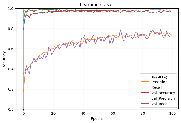
The accuracy metrics of the model on the train data are as follows:

from sklearn.metrics import classification_report, confusion_matrix
y_test_pred = np.where(model.predict(x_test)<0.5, 0, 1)
print(classification_report(y_test, y_test_pred))
print("confusion matrix")
print(confusion_matrix(y_test, y_test_pred))

[1m314/314[0m [32m━━━━━━━━━━━━━━━━━━━━[0m[37m[0m [1m1s[0m 2ms/step
              precision    recall  f1-score   support

           0       1.00      0.98      0.99      9549
           1       0.73      0.97      0.83       487

    accuracy                           0.98     10036
   macro avg       0.86      0.97      0.91     10036
weighted avg       0.99      0.98      0.98     10036

confusion matrix
[[9375  174]
 [  16  471]]

keras.utils.plot_model(model, "absenteeism.png", show_shapes=True)

png

The training accuracy is

y_train_pred = np.where(model.predict(x_train)<0.5, 0, 1)
print(classification_report(y_train, y_train_pred))
print("Confusion metrix")
print(confusion_matrix(y_train, y_train_pred))

[1m732/732[0m [32m━━━━━━━━━━━━━━━━━━━━[0m[37m[0m [1m2s[0m 3ms/step
              precision    recall  f1-score   support

           0       1.00      0.98      0.99     22278
           1       0.77      1.00      0.87      1137

    accuracy                           0.99     23415
   macro avg       0.88      0.99      0.93     23415
weighted avg       0.99      0.99      0.99     23415

Confusion metrix
[[21933   345]
 [    0  1137]]

Saving the model

model.save("my_keras_model.keras")
model.save_weights("my_keras_weights.weights.h5")

The accuracy of this initial model is very good and is very similar to the accuracy in the machine learning blog. But still, can we improve on this accuracy? Let's look at some ways we can improve any neural network model.

Vanishing gradients/exploding gradients problem¶

The backpropagation algorithm works by propagating the error gradient from the outer layer to the lower layers. Sometimes the gradients in the lower layers get smaller and smaller or larger and larger when flowing in DNN during training. This makes the lower layers hard to train.

In the logistic activation function, for example, if the inputs become extremely large or extremely small, the function saturates at 1 or 0 with a derivative close to 0. This means there will be no gradient to propagate back to the lower layers.

To reduce unstable gradients, the variance of the outputs of each layer should be equal to the variance of its inputs (the gradients should also have equal variance) after the forward and backward passes.

Fine-tuning can not only help us find the best parameters but can also help us prevent vanishing or exploding gradients.

Fine-tuning neural network hyperparameters¶

There are multiple hyperparameters in a neural network that can be tweaked, like network architecture, number of hidden layers, number of neurons in each layer, type of activation function, and more. Many libraries can be used to handle these, like hyperopt, hyperas, keras tuner, scikit optimise, spearmint, hyperband, etc. The first step is to create a function that can build and compile a Keras model.

def build_model(n_hidden=1, n_neurons=30, learning_rate=0.001, hidden_layer_activation = 'relu', kernel_initializer = 'he_normal', input_shape=[input_length],
                kernel_regularizer=None, kernel_constraint=None, dropout_rate = 0.1, optimizer='sgd'):
    model = Sequential()
    model.add(InputLayer(input_shape=input_shape))
    model.add(keras.layers.BatchNormalization())
    for layer in range(n_hidden):
        model.add(keras.layers.Dense(n_neurons, activation=hidden_layer_activation, kernel_initializer=kernel_initializer,
                                     kernel_regularizer=kernel_regularizer, kernel_constraint=kernel_constraint))
        model.add(Dropout(rate=dropout_rate))
    model.add(keras.layers.Dense(1, activation='sigmoid'))
    model.compile(loss="binary_crossentropy", metrics=accuracy_metrics, optimizer=optimizer)
    model.optimizer.learning_rate.assign(learning_rate)
    return model

This function demonstrates some of the popular hyperparameters that can be used. Let's look at each one of them:

Number of hidden layers¶

Theoretically, one hidden layer will be able to model any complex function, but it will require many neurons in that layer and will require exponentially more training parameters when compared to deep networks with a smaller number of neurons in each layer. Hierarchical structures help DNNs converge faster and generalize better on new and unseen datasets. The neurons that are in layers closer to the input layer (low-level layers) model low-level structures and higher-level layers build on these low-level structures to build higher-level structures.

Number of neurons per hidden layer¶

There are two approaches to the number of neurons in a hidden layer. One is to stack them like a pyramid, with more neurons at hidden layers close to the input layers and decreasing them up to the output layer. The other is to have the same number of neurons in all layers. I prefer the second method because it is easier to have a larger number of neurons than needed and then to use early stopping and other regularization techniques to prevent overfitting.

Batch size¶

The batch size should be dependent on the type of GPUs and TPUs that are used. For regular datasets, a batch size of 32 is most optimal. Larger batch sizes have faster training but do not converge faster, while smaller batch sizes converge in a smaller number of epochs, but each epoch takes longer to train.

Activation function¶

For output neurons, the activation functions are as follows:

Problem Type	Output layer activation functions
Binary classification	Logistic
Multiclass classification	Softmax
Regression	None,ReLU/softplus(+vs outputs), logistic/tanh(bounded outputs)

For regular DNNs, the activation function for hidden neurons is generally ReLU. ReLU's face issues known as dying RELU, where they output only 0. There are several varieties of ReLU to solve this problem.

Leaky Relu¶

In Leaky ReLU, a hyperparameter $\alpha$ defines the slope of the function for negative values of z. This is called a leak, which prevents ReLUs from dying. $$ LeakyReLU(z) = max(\alpha z, z)$$

SELU¶

The scaled Exponential Linear Unit is the best variant of ReLU, where an exponential function is used for negative input values in such a way that the slope at 0 is non-zero.

\[ ELU_{\alpha}(z) =\begin{cases} \alpha(exp(z)-1) & z < 0 \\ z & z \geq 0 \end{cases} \]

IIf a deep neural network consists of only SELUs as the activation function in all of the hidden layers, the data will self-normalize. The output of every layer will have a mean of zero and a standard deviation of one. This will reduce the vanishing gradients problem.

Optimizer¶

The optimizer used also changes the speed of training. Apart from gradient descent, another popular optimizer is the Adam optimizer.

Batch normalisation¶

The normalization layer normalizes the input data in such a way that the mean of the input is zero and the standard deviation is one. This can prevent the vanishing gradient issue as it forces the input and output variances to be constant at one.

Weight initialisation¶

Garot and He initialization can be used to initialize the weights in the network in such a way that the vanishing and exploding gradients can be reduced.

Initialization	Activation functions
Glorot	None, Tanh, Logistic, Softmax
He	ReLU and variants
LeCun	SELU

Gradient clipping¶

One way to reduce the vanishing gradient problem is to clip the gradients so that they never exceed a threshold during backpropagation.

Regularization (l1 and l2)¶

L1 regularizations can be applied to the gradients to constrain the weights of the network. L2 regularization can force many weights to be zero, making a sparse network. These can help in regularizing the weights of the network.

One of the ways to find the optimized parameters is to use Grid Search CV for a smaller number of epochs and then train the best model until stopping criteria is met.

from scikeras.wrappers import KerasClassifier
keras_reg = KerasClassifier(model=build_model, epochs=25, batch_size=32, verbose=2)

from sklearn.model_selection import RandomizedSearchCV, GridSearchCV

param_distribs = {
    "model__n_hidden": [3],
    "model__n_neurons": [30],
    "model__learning_rate": [0.01, 0.001],
    "model__hidden_layer_activation": ['relu', "elu"],
    "model__kernel_initializer":["he_normal", "lecun_normal", keras.initializers.VarianceScaling(scale=2., mode='fan_avg', distribution='uniform')],
    "model__kernel_regularizer":[None, keras.regularizers.l2(0.01)],
    "model__kernel_constraint":[None, keras.constraints.max_norm(1.)],
    "model__dropout_rate":[0.1, 0.2],
    "model__optimizer":['adam', "sgd", keras.optimizers.SGD(clipvalue=1.0), keras.optimizers.SGD(clipnorm=1.0)],
    "batch_size":[32, 1000],
    "epochs":[50],
}

rnd_search_cv = GridSearchCV(keras_reg, param_distribs, cv=5, verbose=2)
rnd_search_cv.fit(x_train, y_train, validation_data=(x_test, y_test), class_weight = class_weights)

Fitting 5 folds for each of 768 candidates, totalling 3840 fits

Epoch 1/50
19/19 - 13s - 678ms/step - Precision: 0.0542 - Recall: 0.0945 - accuracy: 0.8759 - fn: 986.0000 - fp: 5238.0000 - loss: 1.8458 - tn: 39955.0000 - tp: 1321.0000 - val_Precision: 0.0480 - val_Recall: 0.0554 - val_accuracy: 0.9009 - val_fn: 460.0000 - val_fp: 535.0000 - val_loss: 0.3782 - val_tn: 9014.0000 - val_tp: 27.0000
Epoch 2/50
19/19 - 0s - 10ms/step - Precision: 0.0507 - Recall: 0.1473 - accuracy: 0.8246 - fn: 776.0000 - fp: 2510.0000 - loss: 1.6876 - tn: 15312.0000 - tp: 134.0000 - val_Precision: 0.0590 - val_Recall: 0.1417 - val_accuracy: 0.8486 - val_fn: 418.0000 - val_fp: 1101.0000 - val_loss: 0.4418 - val_tn: 8448.0000 - val_tp: 69.0000
...
Epoch 49/50
19/19 - 0s - 7ms/step - Precision: 0.1297 - Recall: 0.7703 - accuracy: 0.7377 - fn: 209.0000 - fp: 4704.0000 - loss: 1.0418 - tn: 13118.0000 - tp: 701.0000 - val_Precision: 0.1510 - val_Recall: 0.8604 - val_accuracy: 0.7586 - val_fn: 68.0000 - val_fp: 2355.0000 - val_loss: 0.5031 - val_tn: 7194.0000 - val_tp: 419.0000
Epoch 50/50
19/19 - 0s - 6ms/step - Precision: 0.1290 - Recall: 0.7659 - accuracy: 0.7373 - fn: 213.0000 - fp: 4708.0000 - loss: 1.0323 - tn: 13114.0000 - tp: 697.0000 - val_Precision: 0.1520 - val_Recall: 0.8645 - val_accuracy: 0.7594 - val_fn: 66.0000 - val_fp: 2349.0000 - val_loss: 0.4998 - val_tn: 7200.0000 - val_tp: 421.0000
5/5 - 0s - 70ms/step
[CV] END batch_size=1000, epochs=50, model__hidden_layer_activation=relu, model__kernel_regularizer=None, model__n_hidden=3, model__n_neurons=30; total time=  26.2s
Epoch 1/50
...
[CV] END batch_size=1000, epochs=50, model__hidden_layer_activation=relu, model__kernel_regularizer=None, model__n_hidden=3, model__n_neurons=30; total time=  22.0s
Epoch 1/50
...
...
Epoch 49/50
24/24 - 0s - 12ms/step - Precision: 0.1745 - Recall: 0.8751 - accuracy: 0.7929 - fn: 142.0000 - fp: 4708.0000 - loss: 0.7878 - tn: 17570.0000 - tp: 995.0000 - val_Precision: 0.1963 - val_Recall: 0.9671 - val_accuracy: 0.8062 - val_fn: 16.0000 - val_fp: 1929.0000 - val_loss: 0.4336 - val_tn: 7620.0000 - val_tp: 471.0000
Epoch 50/50
24/24 - 0s - 12ms/step - Precision: 0.1766 - Recall: 0.8865 - accuracy: 0.7938 - fn: 129.0000 - fp: 4700.0000 - loss: 0.7704 - tn: 17578.0000 - tp: 1008.0000 - val_Precision: 0.1986 - val_Recall: 0.9671 - val_accuracy: 0.8090 - val_fn: 16.0000 - val_fp: 1901.0000 - val_loss: 0.4287 - val_tn: 7648.0000 - val_tp: 471.0000

GridSearchCV(cv=5,
             estimator=KerasClassifier(batch_size=32, epochs=25, model=<function build_model at 0x7b760e5b67a0>, verbose=2),
             param_grid={'batch_size': [1000], 'epochs': [50],
                         'model__hidden_layer_activation': ['relu', 'elu'],
                         'model__kernel_regularizer': [None,
                                                       <keras.src.regularizers.regularizers.L2 object at 0x7b760de7ed40>],
                         'model__n_hidden': [3], 'model__n_neurons': [30]},
             verbose=2)

In a Jupyter environment, please rerun this cell to show the HTML representation or trust the notebook.
On GitHub, the HTML representation is unable to render, please try loading this page with nbviewer.org.

The best model is

rnd_search_cv.best_estimator_

KerasClassifier(
    model=<function build_model at 0x7b760e5b67a0>
    build_fn=None
    warm_start=False
    random_state=None
    optimizer=rmsprop
    loss=None
    metrics=None
    batch_size=1000
    validation_batch_size=None
    verbose=2
    callbacks=None
    validation_split=0.0
    shuffle=True
    run_eagerly=False
    epochs=50
    class_weight=None
    model__hidden_layer_activation=elu
    model__kernel_regularizer=None
    model__n_hidden=3
    model__n_neurons=30
)

rnd_search_cv.best_params_

{'batch_size': 1000,
 'epochs': 50,
 'model__hidden_layer_activation': 'elu',
 'model__kernel_regularizer': None,
 'model__n_hidden': 3,
 'model__n_neurons': 30}

Accuracy metrics for the best model are:

rnd_search_cv.best_score_

0.792568866111467

rnd_search_cv.score(x_test, y_test)

11/11 - 0s - 33ms/step
0.8089876444798725

Training the best model¶

Once we find the best hyperparameters, we can use those to further train the model.

Learning rate scheduling¶

A very high learning rate might diverge and never reach optimum while a small learning rate will take a long time to arrive at A very high learning rate might diverge and never reach optimum, while a small learning rate will take a long time to reach optimum. Instead, we can train the model with a large learning rate at first and then gradually cross epochs. Reduce Learning Rate on Plateau is a method where the learning rate is reduced by a factor once the loss function stagnates.

Early stopping and model checkpoints¶

Model checkpoints and early stopping can be used when training a large number of epochs. Early stopping is a stopping criterion to stop training when the loss metric stagnates. Additionally, model checkpoints can also help in resuming training from the last saved point in case of interruptions or failures during the training process. This ensures that the training progress is not lost and can be continued seamlessly.

lr_scheduler = keras.callbacks.ReduceLROnPlateau(factor=0.05, patience=10)
early_stopping = keras.callbacks.EarlyStopping(patience=10, min_delta=0)
checkpoint_cb = keras.callbacks.ModelCheckpoint("my_optimised_keras_model.keras", save_best_only=True)

model2 = rnd_search_cv.best_estimator_.model_
history = model2.fit(x_train, y_train, class_weight = class_weights,
                    validation_data=(x_test, y_test),
                    callbacks=[checkpoint_cb, early_stopping, lr_scheduler],
                    epochs=1000, batch_size=rnd_search_cv.best_estimator_.batch_size)

Epoch 1/1000
[1m24/24[0m [32m━━━━━━━━━━━━━━━━━━━━[0m[37m[0m [1m11s[0m 249ms/step - Precision: 0.1848 - Recall: 0.9000 - accuracy: 0.8013 - fn: 67.6000 - fp: 2496.9199 - loss: 0.7515 - tn: 9787.3604 - tp: 561.3200 - val_Precision: 0.2011 - val_Recall: 0.9671 - val_accuracy: 0.8120 - val_fn: 16.0000 - val_fp: 1871.0000 - val_loss: 0.4257 - val_tn: 7678.0000 - val_tp: 471.0000 - learning_rate: 0.0010  
...  
Epoch 156/1000
[1m24/24[0m [32m━━━━━━━━━━━━━━━━━━━━[0m[37m[0m [1m0s[0m 15ms/step - Precision: 0.3215 - Recall: 0.9418 - accuracy: 0.9013 - fn: 36.9600 - fp: 1237.6000 - loss: 0.4189 - tn: 11053.1602 - tp: 585.4800 - val_Precision: 0.3214 - val_Recall: 0.9795 - val_accuracy: 0.8987 - val_fn: 10.0000 - val_fp: 1007.0000 - val_loss: 0.2359 - val_tn: 8542.0000 - val_tp: 477.0000 - learning_rate: 0.0010
Epoch 157/1000
[1m24/24[0m [32m━━━━━━━━━━━━━━━━━━━━[0m[37m[0m [1m1s[0m 18ms/step - Precision: 0.3173 - Recall: 0.9483 - accuracy: 0.8995 - fn: 34.7600 - fp: 1247.2000 - loss: 0.4196 - tn: 11047.0801 - tp: 584.1600 - val_Precision: 0.3212 - val_Recall: 0.9795 - val_accuracy: 0.8986 - val_fn: 10.0000 - val_fp: 1008.0000 - val_loss: 0.2365 - val_tn: 8541.0000 - val_tp: 477.0000 - learning_rate: 0.0010
Epoch 158/1000
[1m24/24[0m [32m━━━━━━━━━━━━━━━━━━━━[0m[37m[0m [1m1s[0m 12ms/step - Precision: 0.3330 - Recall: 0.9419 - accuracy: 0.9040 - fn: 35.3600 - fp: 1211.6000 - loss: 0.4260 - tn: 11074.6797 - tp: 591.5600 - val_Precision: 0.3210 - val_Recall: 0.9795 - val_accuracy: 0.8985 - val_fn: 10.0000 - val_fp: 1009.0000 - val_loss: 0.2369 - val_tn: 8540.0000 - val_tp: 477.0000 - learning_rate: 0.0010
Epoch 159/1000
[1m24/24[0m [32m━━━━━━━━━━━━━━━━━━━━[0m[37m[0m [1m0s[0m 13ms/step - Precision: 0.3331 - Recall: 0.9570 - accuracy: 0.9031 - fn: 27.6000 - fp: 1231.7200 - loss: 0.4086 - tn: 11051.5195 - tp: 602.3600 - val_Precision: 0.3212 - val_Recall: 0.9795 - val_accuracy: 0.8986 - val_fn: 10.0000 - val_fp: 1008.0000 - val_loss: 0.2365 - val_tn: 8541.0000 - val_tp: 477.0000 - learning_rate: 0.0010
Epoch 160/1000
[1m24/24[0m [32m━━━━━━━━━━━━━━━━━━━━[0m[37m[0m [1m0s[0m 6ms/step - Precision: 0.3231 - Recall: 0.9429 - accuracy: 0.9010 - fn: 31.8000 - fp: 1237.9200 - loss: 0.4298 - tn: 11047.8799 - tp: 595.6000 - val_Precision: 0.3223 - val_Recall: 0.9795 - val_accuracy: 0.8991 - val_fn: 10.0000 - val_fp: 1003.0000 - val_loss: 0.2358 - val_tn: 8546.0000 - val_tp: 477.0000 - learning_rate: 0.0010

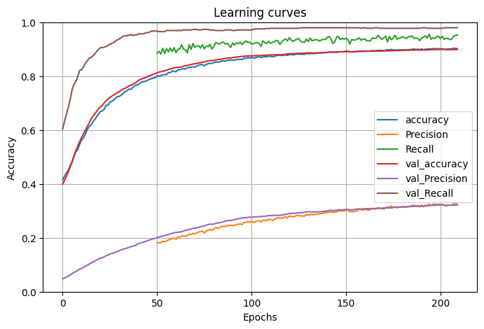
Accuracy metrics and error

pd.concat([pd.DataFrame(rnd_search_cv.best_estimator_.history_), pd.DataFrame(history.history)]).reset_index()[['accuracy', 'Precision', 'Recall', 'val_accuracy', 'val_Precision', 'val_Recall']].plot(figsize=(8, 5))
plt.grid(True)
plt.gca().set_ylim(0, 1)
plt.xlabel("Epochs")
plt.ylabel("Accuracy")
plt.title("Learning curves")
plt.show()

png

y_test_pred = np.where(model2.predict(x_test)<0.5, 0, 1)
print(classification_report(y_test, y_test_pred))
print("Confusion matrix")
print(confusion_matrix(y_test, y_test_pred))

[1m314/314[0m [32m━━━━━━━━━━━━━━━━━━━━[0m[37m[0m [1m1s[0m 2ms/step
              precision    recall  f1-score   support

           0       1.00      0.89      0.94      9549
           1       0.32      0.98      0.49       487

    accuracy                           0.90     10036
   macro avg       0.66      0.94      0.71     10036
weighted avg       0.97      0.90      0.92     10036

Confusion matrix
[[8546 1003]
 [  10  477]]

Loading the best model that is saved

loaded_model = keras.models.load_model("my_optimised_keras_model.keras")

y_test_pred = np.where(loaded_model.predict(x_test)<0.5, 0, 1)
print(classification_report(y_test, y_test_pred))
print(confusion_matrix(y_test, y_test_pred))

[1m314/314[0m [32m━━━━━━━━━━━━━━━━━━━━[0m[37m[0m [1m1s[0m 2ms/step
              precision    recall  f1-score   support

           0       1.00      0.89      0.94      9549
           1       0.32      0.98      0.48       487

    accuracy                           0.90     10036
   macro avg       0.66      0.94      0.71     10036
weighted avg       0.97      0.90      0.92     10036

[[8545 1004]
 [  11  476]]

The accuracy of the trained model is very similar to that of the Scikit-Learn model.

References¶

GeÌron, A. (2019). Hands-on machine learning with Scikit-Learn, Keras and TensorFlow: concepts, tools, and techniques to build intelligent systems (2^nd ed.). O’Reilly.
Class notes: Business Analytics & Intelligence (BAI –10): Prof Naveen Kumar Bhansali
https://github.com/ageron/handson-ml2