BabyGrootGPT: A Guided Walkthrough of the Transformer Decoder From Scratch
1. The Problem We Are Solving
This notebook is not trying to build a production language model. It is trying to make a Transformer decoder easy to see.
Our goal is to answer one concrete question: how does a decoder-only model take a short prompt, represent it numerically, route information across tokens, and predict the next token without looking into the future?
That question is hard to understand in a large model because the key ideas sit under large vocabularies, deep stacks of layers, and millions of parameters. So we shrink the setting on purpose.
Why use a toy dataset?
We train on a tiny corpus of 19 short sentences and end up with a vocabulary of just 24 tokens, including <PAD>, <START>, and <END>. That small setup is a feature, not a limitation.
With a 24-token vocabulary, we can inspect the full token dictionary, the embedding tables, the padded training pairs, the attention matrix, and the final logits without getting lost in scale. Every major tensor is small enough to print, reason about, and connect back to the maths.
This means the notebook can focus on intuition:
- how raw text becomes token IDs
- how autoregressive training examples are created
- how self-attention mixes context
- how logits become next-token predictions
Once that pipeline is clear in a toy setting, the same ideas transfer directly to larger Transformer decoders.
RNNs vs Transformer Decoders
Traditional sequence models such as RNNs and LSTMs process text one token at a time:
Each hidden state must pass through the next step in order. That makes training slower, limits parallelism, and makes long-range dependencies harder to preserve.
Transformer decoders replace recurrence with self-attention. Instead of waiting for tokens to arrive one by one, the model ingests the available sequence together, computes query-key-value interactions in parallel, and then uses a causal mask so each position can only attend to itself and earlier tokens.
In other words:
- RNN/LSTM: sequential state passing
- Transformer decoder: parallel context scoring with masked next-token prediction
That contrast is the core motivation for the notebook. We want to see exactly how a masked self-attention system does the job that older sequential models handled through recurrence.
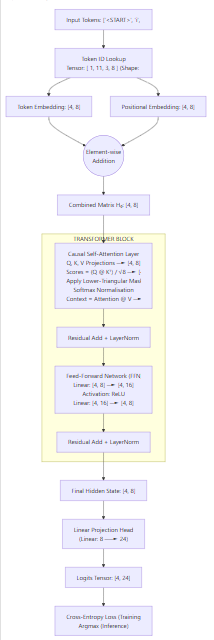
2. End-to-End Architecture Flow
Input Tokens: ["<START>", "i", "am", "groot"]
                         │
                         ▼
             [ Token ID Lookup ] ───► Tensor: [ 1, 11, 3, 8 ] (Shape: [4])
                         │
        ┌────────────────┴────────────────┐
        ▼                                 ▼
Token Embedding: [4, 8]        Positional Embedding: [4, 8]
        └────────────────┬────────────────┘
                         ▼  (Element-wise Addition)
              Combined Matrix H₀: [4, 8]
                         │
                         ▼
           ╔═════════════════════════════════════════╗
           ║            TRANSFORMER BLOCK            ║
           ║                                         ║
           ║  ┌───────────────────────────────────┐  ║
           ║  │    Causal Self-Attention Layer    │  ║
           ║  │  Q, K, V Projections ──► [4, 8]   │  ║
           ║  │  Scores = (Q @ Kᵀ) / √8 ──► [4, 4]│  ║
           ║  │  Apply Lower-Triangular Mask      │  ║
           ║  │  Softmax Normalisation            │  ║
           ║  │  Context = Attention @ V ──►[4, 8]│  ║
           ║  └─────────────────┬─────────────────┘  ║
           ║                    ▼                    ║
           ║       Residual Add + LayerNorm          ║
           ║                    │                    ║
           ║  ┌─────────────────┴─────────────────┐  ║
           ║  │     Feed-Forward Network (FFN)    │  ║
           ║  │     Linear: [4, 8] ──► [4, 16]    │  ║
           ║  │     Activation: ReLU              │  ║
           ║  │     Linear: [4, 16] ──► [4, 8]    │  ║
           ║  └─────────────────┬─────────────────┘  ║
           ║                    ▼                    ║
           ║       Residual Add + LayerNorm          ║
           ╚════════════════════┼════════════════════╝
                                │
                                ▼
                   Final Hidden State: [4, 8]
                                │
                                ▼
         [ Linear Projection Head (Linear: 8 ──► 24) ]
                                │
                                ▼
                    Logits Tensor: [4, 24]
                                │
                                ▼
      [ Cross-Entropy Loss (Training) / Argmax (Inference) ]
Reading Roadmap
This article is organised in two passes. The first pass builds the decoder from a tiny text world up to next-token prediction. The second pass revisits the same machinery with deeper matrix-level inspection.
3. How to Read This Guide
The walkthrough below is organised into seven parts. Each part introduces one segment of the decoder pipeline, explains why it exists, shows the math in context, and then runs the exact code that produces the tensors and outputs.
Part 1 (Data Setup): corpus, vocabulary, token IDs, and padded autoregressive training pairs.Part 2 (Model & Immediate Training): the PyTorch modules and the first full training run.Part 3 (The Interludes): one traced sequence through the learned embedding and input matrices.Part 4 (Self Attention Layer): queries, keys, values, scaled dot products, masking, and context mixing.Part 5 (Tracing the Matrix Through the Transformer Block): residual connections, layer normalisation, and the FFN path.Part 6 (Logits, Probabilities, and Generation): the output head, softmax probabilities, and greedy decoding.Part 7 (Final Output and Summary): end-to-end generation behaviour and the main decoder takeaways.
Part 1: Data Setup
Before we build the neural network, we must load our tools, define a local display helper, and prepare our language. We use PyTorch as our deep learning framework to handle matrix operations and construct neural layers.
import torch
import torch.nn as nn
import torch.nn.functional as F
import pandas as pd
import numpy as np
import matplotlib.pyplot as plt
import seaborn as sns
from IPython.display import display
from baby_groot_viz import *

torch.manual_seed(42)
device = "cuda" if torch.cuda.is_available() else "cpu"
print(f"Using device: {device}")
Using device: cpu
Neural networks cannot process raw text; they strictly perform mathematical operations on numbers. So we first create a tiny corpus that is intentionally small enough to inspect end to end. From that corpus, we build a vocabulary that assigns one integer ID to every unique token the model is allowed to know.
This is why the vocabulary size of 24 matters. It is large enough to include repeated patterns such as groot likes tree, tree needs water, and rocket helps groot, but small enough that we can still print the entire lookup table and understand what the model is doing at each stage.
We also introduce three structural tokens:
<PAD>(ID 0): Used to fill empty spaces so all sentences reach a uniform length.<START>(ID 1): Acts as a cue, telling the model to begin generating a sentence.<END>(ID 2): The model learns to output this token when the sentence is complete.
Conceptual Input & Output
Input (Raw Text Corpus):
"i am groot"
"you are groot"
"we are groot"
...


```python
corpus = [
    "i am groot",
    "you are groot",
    "we are groot",
    "groot is happy",
    "groot is sad",
    "groot is angry",
    "happy groot smiles",
    "sad groot cries",
    "angry groot shouts",
    "groot likes tree",
    "groot likes leaf",
    "tree needs water",
    "leaf needs water",
    "water helps tree",
    "tree helps groot",
    "groot helps rocket",
    "rocket helps groot",
    "groot likes friend",
    "friend likes groot"
]

special_tokens = ["<PAD>", "<START>", "<END>"]

words = set()
for sentence in corpus:
    for word in sentence.split():
        words.add(word)

vocab = special_tokens + sorted(list(words))
token_to_id = {token: idx for idx, token in enumerate(vocab)}
id_to_token = {idx: token for token, idx in token_to_id.items()}
vocab_size = len(vocab)

print(f"Vocabulary Size: {vocab_size}")
Vocabulary Size: 24
Output (Vocabulary Dictionary): The model scans the corpus, extracts 21 unique words, and adds the 3 special tokens, resulting in a total vocabulary size of 24.
show_vocabulary(token_to_id)
Token        | Token ID
-----------------------
<PAD>        | 0
<START>      | 1
<END>        | 2
am           | 3
angry        | 4
are          | 5
cries        | 6
friend       | 7
groot        | 8
happy        | 9
helps        | 10
i            | 11
is           | 12
leaf         | 13
likes        | 14
needs        | 15
rocket       | 16
sad          | 17
shouts       | 18
smiles       | 19
tree         | 20
water        | 21
we           | 22
you          | 23
Step 2: Autoregressive Data Construction and Padding
To teach the model how to write, we train it autoregressively. Each training row asks the model to predict the next token \(y_t\) from the prior context \(x_{1:t-1}\).
Because neural networks require uniform tensors, we pad each context row to the maximum context length.
When we pass a sentence to the model, we first bracket it with our special start and end tokens, then map it through the vocabulary dictionary into an integer vector (a 1D matrix):
Consider the integer-mapped sequence for <START> i am groot <END> $\(\text{["<START>", "i", "am", "groot", "<END>"]} \quad \xrightarrow{\text{Tokenisation}} \quad \begin{bmatrix} 1 & 11 & 3 & 8 & 2 \end{bmatrix}\)$
We break this single sequence into four distinct training examples. We pad the inputs with 0 until they all reach the maximum length of 4.
| Step | Raw Context | Target | Padded Context Matrix (\(\mathbf{X}\)) | Target ID (\(\mathbf{Y}\)) |
|---|---|---|---|---|
| 1 | <START> | i | \(\begin{bmatrix} 1 & 0 & 0 & 0 \end{bmatrix}\) | 11 |
| 2 | <START> i | am | \(\begin{bmatrix} 1 & 11 & 0 & 0 \end{bmatrix}\) | 3 |
| 3 | <START> i am | groot | \(\begin{bmatrix} 1 & 11 & 3 & 0 \end{bmatrix}\) | 8 |
| 4 | <START> i am groot | <END> | \(\begin{bmatrix} 1 & 11 & 3 & 8 \end{bmatrix}\) | 2 |
After processing all 19 sentences in the corpus, we stack these 1D arrays into 2D matrices (Tensors). The entire training dataset results in 76 flashcards.
-
\(\mathbf{X}\) Tensor (Input Contexts): Shape
[76, 4](76 examples, each containing 4 tokens). -
\(\mathbf{Y}\) Tensor (Targets): Shape
[76](76 single-token answers).
encoded_sentences = []
for sentence in corpus:
    tokens = ["<START>"] + sentence.split() + ["<END>"]
    ids = [token_to_id[token] for token in tokens]
    encoded_sentences.append(ids)

X = []
Y = []
for ids in encoded_sentences:
    for i in range(1, len(ids)):
        X.append(ids[:i])
        Y.append(ids[i])

max_len = max(len(x) for x in X)
pad_id = token_to_id["<PAD>"]

X_padded = []
for seq in X:
    padded = seq + [pad_id] * (max_len - len(seq))
    X_padded.append(padded)

X_tensor = torch.tensor(X_padded)
Y_tensor = torch.tensor(Y)

print("Input shape (X_tensor):", X_tensor.shape)
print("Target shape (Y_tensor):", Y_tensor.shape)

dataset = torch.utils.data.TensorDataset(X_tensor, Y_tensor)
loader = torch.utils.data.DataLoader(dataset, batch_size=16, shuffle=True)
Input shape (X_tensor): torch.Size([76, 4])
Target shape (Y_tensor): torch.Size([76])
show_training_pairs(X_tensor, Y_tensor, id_to_token)
First 15 training pairs:
| Sample | X (IDs) | X (Tokens) | Y (ID) | Y (Target Token) | |
|---|---|---|---|---|---|
| 0 | 1 | [1, 0, 0, 0] | <START> <PAD> <PAD> <PAD> | 11 | i |
| 1 | 2 | [1, 11, 0, 0] | <START> i <PAD> <PAD> | 3 | am |
| 2 | 3 | [1, 11, 3, 0] | <START> i am <PAD> | 8 | groot |
| 3 | 4 | [1, 11, 3, 8] | <START> i am groot | 2 | <END> |
| 4 | 5 | [1, 0, 0, 0] | <START> <PAD> <PAD> <PAD> | 23 | you |
| 5 | 6 | [1, 23, 0, 0] | <START> you <PAD> <PAD> | 5 | are |
| 6 | 7 | [1, 23, 5, 0] | <START> you are <PAD> | 8 | groot |
| 7 | 8 | [1, 23, 5, 8] | <START> you are groot | 2 | <END> |
| 8 | 9 | [1, 0, 0, 0] | <START> <PAD> <PAD> <PAD> | 22 | we |
| 9 | 10 | [1, 22, 0, 0] | <START> we <PAD> <PAD> | 5 | are |
| 10 | 11 | [1, 22, 5, 0] | <START> we are <PAD> | 8 | groot |
| 11 | 12 | [1, 22, 5, 8] | <START> we are groot | 2 | <END> |
| 12 | 13 | [1, 0, 0, 0] | <START> <PAD> <PAD> <PAD> | 8 | groot |
| 13 | 14 | [1, 8, 0, 0] | <START> groot <PAD> <PAD> | 12 | is |
| 14 | 15 | [1, 8, 12, 0] | <START> groot is <PAD> | 9 | happy |
Part 2: Model & Immediate Training
This section combines the full decoder architecture into one modular build, then trains it immediately. That ordering matters because the next section inspects learned embeddings, projections, and attention weights.
2.1: Build the Decoder Modules
class CausalSelfAttention(nn.Module):
    def __init__(self, embed_dim):
        super().__init__()
        self.q = nn.Linear(embed_dim, embed_dim)
        self.k = nn.Linear(embed_dim, embed_dim)
        self.v = nn.Linear(embed_dim, embed_dim)

    def forward(self, x):
        B, T, C = x.shape
        Q = self.q(x)
        K = self.k(x)
        V = self.v(x)

        scores = Q @ K.transpose(-2, -1)
        scores = scores / (C ** 0.5)

        mask = torch.tril(torch.ones(T, T, device=x.device))
        scores = scores.masked_fill(mask == 0, -1e9)

        attn = torch.softmax(scores, dim=-1)
        out = attn @ V
        return out, attn


class TransformerBlock(nn.Module):
    def __init__(self, embed_dim):
        super().__init__()
        self.attn = CausalSelfAttention(embed_dim)
        self.norm1 = nn.LayerNorm(embed_dim)
        self.norm2 = nn.LayerNorm(embed_dim)
        self.ffn = nn.Sequential(
            nn.Linear(embed_dim, 16),
            nn.ReLU(),
            nn.Linear(16, embed_dim)
        )

    def forward(self, x):
        attn_out, attn = self.attn(x)
        x = self.norm1(x + attn_out)
        ff_out = self.ffn(x)
        x = self.norm2(x + ff_out)
        return x, attn


class BabyGrootGPT(nn.Module):
    def __init__(self, vocab_size, max_len, embed_dim=8):
        super().__init__()
        self.token_embedding = nn.Embedding(vocab_size, embed_dim)
        self.position_embedding = nn.Embedding(max_len, embed_dim)
        self.transformer = TransformerBlock(embed_dim)
        self.head = nn.Linear(embed_dim, vocab_size)

    def forward(self, x):
        B, T = x.shape
        positions = torch.arange(T, device=x.device).unsqueeze(0)
        token_emb = self.token_embedding(x)
        pos_emb = self.position_embedding(positions)
        h = token_emb + pos_emb
        h, attn = self.transformer(h)
        logits = self.head(h)
        return logits, attn


model = BabyGrootGPT(vocab_size=vocab_size, max_len=max_len, embed_dim=8).to(device)
print(model)
BabyGrootGPT(
  (token_embedding): Embedding(24, 8)
  (position_embedding): Embedding(4, 8)
  (transformer): TransformerBlock(
    (attn): CausalSelfAttention(
      (q): Linear(in_features=8, out_features=8, bias=True)
      (k): Linear(in_features=8, out_features=8, bias=True)
      (v): Linear(in_features=8, out_features=8, bias=True)
    )
    (norm1): LayerNorm((8,), eps=1e-05, elementwise_affine=True, bias=True)
    (norm2): LayerNorm((8,), eps=1e-05, elementwise_affine=True, bias=True)
    (ffn): Sequential(
      (0): Linear(in_features=8, out_features=16, bias=True)
      (1): ReLU()
      (2): Linear(in_features=16, out_features=8, bias=True)
    )
  )
  (head): Linear(in_features=8, out_features=24, bias=True)
)
Step 4: Train the Decoder and Plot the Loss
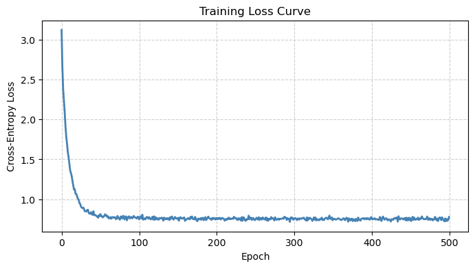
The training loop uses cross-entropy loss on the last real token before padding begins.
optimizer = torch.optim.Adam(model.parameters(), lr=0.01)
losses = []
epochs = 500

for epoch in range(epochs):
    total_loss = 0

    for x, y in loader:
        x = x.to(device)
        y = y.to(device)

        logits, _ = model(x)
        lengths = (x != pad_id).sum(dim=1)
        last_logits = logits[
            torch.arange(x.size(0), device=x.device),
            lengths - 1
        ]

        loss = F.cross_entropy(last_logits, y)

        optimizer.zero_grad()
        loss.backward()
        optimizer.step()

        total_loss += loss.item()

    avg_loss = total_loss / len(loader)
    losses.append(avg_loss)

    if epoch % 50 == 0:
        print(f"Epoch {epoch:3d} | Loss: {avg_loss:.4f}")

plt.figure(figsize=(8, 4))
plt.plot(losses, color="steelblue", lw=2)
plt.title("Training Loss Curve")
plt.xlabel("Epoch")
plt.ylabel("Cross-Entropy Loss")
plt.grid(True, linestyle="--", alpha=0.6)
plt.show();
Epoch   0 | Loss: 3.1198
Epoch  50 | Loss: 0.8143
Epoch 100 | Loss: 0.7484
Epoch 150 | Loss: 0.7672
Epoch 200 | Loss: 0.7508
Epoch 250 | Loss: 0.7477
Epoch 300 | Loss: 0.7627
Epoch 350 | Loss: 0.7492
Epoch 400 | Loss: 0.7485
Epoch 450 | Loss: 0.7264
Part 3: The Interludes
The next three interludes slow the model down and inspect one trained sequence, "<START> i am groot", at matrix level. Every tensor in this part keeps explicit token labels and rounded values so the decoder path stays readable.
3.1 Visualising the Embedding Matrices
Before the data ever reaches the Self-Attention mechanism, it must be converted from integers into continuous mathematical vectors. In PyTorch, nn.Embedding acts as a simple lookup table.
# Token embeddings
sentence = ["<START>", "i", "am", "groot"]

show_embeddings(token_to_id, sentence, device, model, vocab_size, id_to_token)
| Word | ID | Emb_1 | Emb_2 | Emb_3 | Emb_4 | Emb_5 | Emb_6 | Emb_7 | Emb_8 | |
|---|---|---|---|---|---|---|---|---|---|---|
| 0 | <PAD> | 0 | 1.93 | 1.49 | 0.90 | -2.11 | 0.68 | -1.23 | -0.04 | -1.60 |
| 1 | <START> | 1 | -0.87 | 0.88 | -0.43 | -0.94 | -0.83 | -0.41 | -0.75 | 0.39 |
| 2 | <END> | 2 | 1.64 | -0.16 | -0.50 | 0.44 | -0.76 | 1.08 | 0.80 | 1.68 |
| 3 | am | 3 | 1.36 | 1.21 | -0.26 | 1.09 | -0.41 | 0.46 | -0.32 | 1.13 |
| 4 | angry | 4 | -0.87 | -1.54 | -1.00 | 2.23 | 0.30 | 0.24 | -0.05 | -1.88 |
| 5 | are | 5 | -2.23 | 0.89 | -1.28 | 0.92 | -1.56 | 1.92 | -1.39 | 0.08 |
| 6 | cries | 6 | -1.33 | -0.37 | 0.88 | 0.61 | 0.03 | 0.57 | -1.06 | -0.63 |
| 7 | friend | 7 | -0.52 | 0.10 | 0.19 | 1.32 | -0.60 | 1.97 | -0.93 | -0.40 |
| 8 | groot | 8 | 1.34 | 1.31 | 2.08 | 0.88 | 0.53 | -0.61 | -1.24 | 1.06 |
| 9 | happy | 9 | -0.62 | -0.26 | -1.25 | 0.78 | -0.51 | -0.20 | -2.43 | -0.09 |
| 10 | helps | 10 | 0.36 | -0.10 | -1.52 | -0.56 | 0.58 | 0.54 | 0.71 | 0.22 |
| 11 | i | 11 | -0.02 | -0.39 | -0.10 | 0.28 | -1.23 | -0.73 | 2.11 | -0.64 |
| 12 | is | 12 | -2.66 | -0.14 | 1.38 | -0.16 | 0.40 | 0.09 | 1.22 | -0.69 |
| 13 | leaf | 13 | -1.76 | -0.56 | 2.38 | -0.39 | 1.43 | 1.08 | 0.34 | -1.12 |
| 14 | likes | 14 | -1.10 | 0.10 | -0.36 | 0.17 | 0.95 | 0.15 | -1.13 | 0.60 |
| 15 | needs | 15 | -0.67 | 0.78 | 0.59 | 0.96 | 0.54 | 0.32 | 1.74 | 0.53 |
| 16 | rocket | 16 | 1.01 | 1.51 | -1.54 | -0.32 | 0.62 | 0.60 | 0.41 | 1.93 |
| 17 | sad | 17 | 0.87 | 0.24 | -1.14 | 1.14 | -0.41 | 1.05 | -0.86 | 0.82 |
| 18 | shouts | 18 | -0.99 | 0.74 | 1.43 | 1.57 | 0.34 | -0.08 | -0.16 | 0.48 |
| 19 | smiles | 19 | 0.30 | 1.27 | -0.63 | 1.65 | -2.00 | -0.93 | -2.14 | 0.80 |
| 20 | tree | 20 | -1.46 | 1.26 | -0.44 | -0.56 | 0.52 | -0.48 | 0.46 | -0.71 |
| 21 | water | 21 | -2.30 | 1.29 | 1.35 | 0.40 | -0.38 | 0.18 | -0.55 | 2.13 |
| 22 | we | 22 | -0.42 | -0.49 | -1.14 | -1.22 | -1.52 | -1.83 | -0.35 | -1.16 |
| 23 | you | 23 | 0.43 | -1.95 | -1.80 | -0.51 | 0.47 | -0.14 | 1.36 | -0.96 |
3.2. The Positional Embedding Lookup Table
Just like the token embeddings, the positional embeddings are stored as a simple lookup table. Since our maximum sequence length (max_len) is 4, this table will only have 4 rows, each containing an 8-dimensional vector.
Because the self-attention mechanism processes all words at the same time, it has no concept of reading left to right. To the model, "groot likes tree" and "tree likes groot" look identical unless we explicitly tell it which word comes first, second, and third.
We solve this by creating a Positional Embedding matrix. This is a \(4 \times 8\) lookup table where Row 0 represents the first slot in a sentence, Row 1 represents the second slot, and so on. During the forward pass, the vector for Position 0 is added directly to the vector for whichever word appears in Position 0.
We can now extract and visualise this spatial lookup table.
show_positional_embeddings(model, max_len)
Positional Embedding Table
| Position | Emb_1 | Emb_2 | Emb_3 | Emb_4 | Emb_5 | Emb_6 | Emb_7 | Emb_8 | |
|---|---|---|---|---|---|---|---|---|---|
| 0 | 0 | 1.65 | -1.69 | 0.92 | 0.13 | -1.27 | 0.51 | 0.50 | 0.99 |
| 1 | 1 | 0.52 | 2.44 | -0.79 | -1.02 | -0.02 | 1.41 | 1.34 | 0.04 |
| 2 | 2 | -0.54 | -1.05 | -0.25 | -0.85 | 0.10 | 0.35 | -0.20 | -2.18 |
| 3 | 3 | -0.96 | 1.08 | -1.09 | 2.14 | 1.25 | -1.69 | 0.36 | 1.90 |
3.3. Constructing the Input Matrix (\(\mathbf{H}_0\))
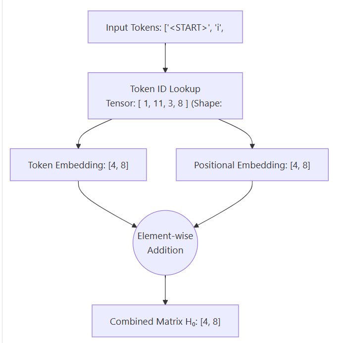
In a Transformer, the true input to the neural network is not just the word, and it is not just the position. It is the element-wise addition of the word's meaning (Token Embedding) and its location in the sentence (Positional Embedding).
We can now extract the exact vectors for the phrase ["<START>", "i", "am", "groot"], add them together, and display the full operation in a clean DataFrame.
Notice how the array under Combined_H0_Vector is the direct sum of the arrays in Token_Embedding and Positional_Encoding.
- Token Embedding Matrix \(\mathbf{E}_{\text{token}}\) (\(4 \times 8\)): Looks up the semantic vector for each token ID.
- Positional Embedding Matrix \(\mathbf{E}_{\text{pos}}\) (\(4 \times 8\)): Looks up the spatial vector for indices \(\begin{bmatrix} 0 & 1 & 2 & 3 \end{bmatrix}\).
ids = [token_to_id[t] for t in sentence]
x_tensor = torch.tensor([ids], device=device)
# H0 trace
with torch.no_grad():
    token_embs = model.token_embedding(x_tensor)[0].cpu().numpy()
    pos_embs = model.position_embedding(torch.arange(len(sentence), device=device)).cpu().numpy()
# Visualise the output
constructing_input_matrix(model, token_to_id, token_embs, pos_embs, ids, id_to_token)
Single-Sequence Input Trace: Token + Position = H_0
| Token | Pos | Token_Embedding | + | Positional_Encoding | = | Combined_H0_Vector | |
|---|---|---|---|---|---|---|---|
| 0 | <START> | 0 | [-0.870, 0.880, -0.430, -0.940, -0.830, -0.410... | + | [1.650, -1.690, 0.920, 0.130, -1.270, 0.510, 0... | = | [0.780, -0.810, 0.490, -0.810, -2.100, 0.100, ... |
| 1 | i | 1 | [-0.020, -0.390, -0.100, 0.280, -1.230, -0.730... | + | [0.520, 2.440, -0.790, -1.020, -0.020, 1.410, ... | = | [0.500, 2.050, -0.890, -0.740, -1.250, 0.680, ... |
| 2 | am | 2 | [1.360, 1.210, -0.260, 1.090, -0.410, 0.460, -... | + | [-0.540, -1.050, -0.250, -0.850, 0.100, 0.350,... | = | [0.820, 0.160, -0.510, 0.240, -0.310, 0.810, -... |
| 3 | groot | 3 | [1.340, 1.310, 2.080, 0.880, 0.530, -0.610, -1... | + | [-0.960, 1.080, -1.090, 2.140, 1.250, -1.690, ... | = | [0.380, 2.390, 0.990, 3.020, 1.780, -2.300, -0... |
H_0 = show_h0(model, token_to_id, sentence, id_to_token, x_tensor, model.token_embedding(x_tensor), model.position_embedding(torch.arange(len(sentence), device=device)))
H_0 Matrix:
| Token | Pos | H0_1 | H0_2 | H0_3 | H0_4 | H0_5 | H0_6 | H0_7 | H0_8 | |
|---|---|---|---|---|---|---|---|---|---|---|
| 0 | <START> | 0 | 0.78 | -0.81 | 0.49 | -0.82 | -2.10 | 0.10 | -0.25 | 1.38 |
| 1 | i | 1 | 0.50 | 2.05 | -0.90 | -0.74 | -1.25 | 0.69 | 3.45 | -0.61 |
| 2 | am | 2 | 0.82 | 0.16 | -0.51 | 0.23 | -0.31 | 0.81 | -0.52 | -1.05 |
| 3 | groot | 3 | 0.38 | 2.39 | 0.98 | 3.02 | 1.78 | -2.30 | -0.88 | 2.96 |
Part 4: Self Attention Layer
Once the model has constructed the \(\mathbf{H}_0\) matrix (the combination of token and positional embeddings), it must figure out how these words relate to each other.
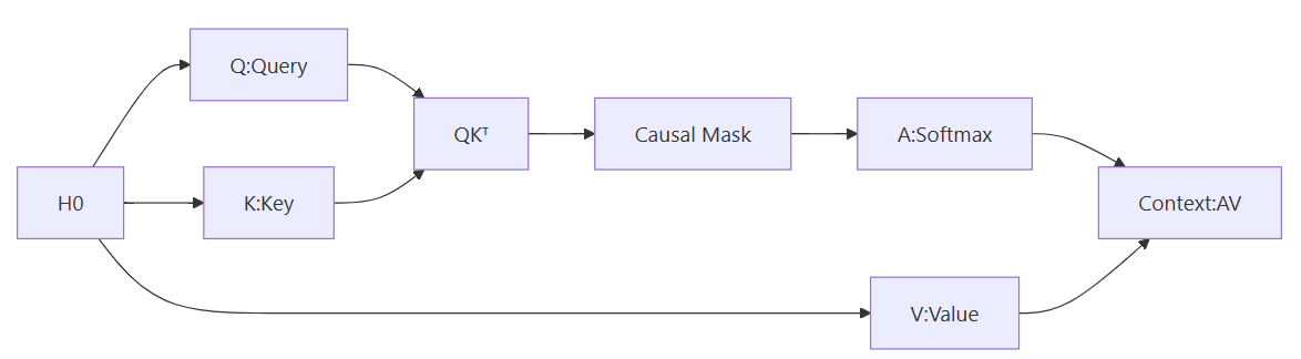
In the Causal Self-Attention layer, the model passes \(\mathbf{H}_0\) through three separate linear transformations (dense neural network layers) to create three new matrices:
- Query (\(\mathbf{Q}\)): Represents what the word is looking for. (e.g., A verb might query for a subject).
- Key (\(\mathbf{K}\)): Represents what the word contains. (e.g., A noun acts as a key for verbs looking for subjects).
- Value (\(\mathbf{V}\)): Represents the actual underlying meaning of the word that will be passed forward if it is selected.
4.1 Generating Queries, Keys, and Values (\(\mathbf{Q}, \mathbf{K}, \mathbf{V}\))
Mathematically, this is done by multiplying \(\mathbf{H}_0\) by the learned weight matrices \(\mathbf{W}_Q\), \(\mathbf{W}_K\), and \(\mathbf{W}_V\), and adding a bias term.
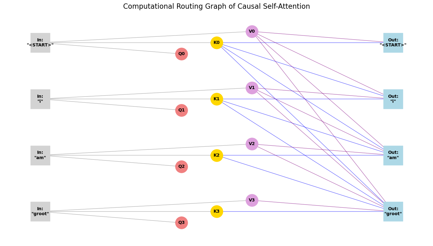
- The Inputs (Left): The combined token and positional embeddings (\(\mathbf{H}_0\)) enter the layer.
- The Split (Middle): Each word branches into three distinct matrices: a Query (Red), a Key (Yellow), and a Value (Purple).
- The Causal Routing (Right): Notice the arrows pointing to the Output node for
"groot". It receives connections from the Keys and Values of<START>,i,am, andgroot. The Output node for<START>only receives connections from its own Key and Value. The missing backward arrows show that the causal mask prevents any look-ahead.
We can now extract the exact Query matrix (\(\mathbf{Q}\)) for our "<START> i am groot" sequence and display it.
display_q_matrix(model, sentence, device, id_to_token, token_to_id)
Query (Q) Matrix:
| Token | Pos | Q_1 | Q_2 | Q_3 | Q_4 | Q_5 | Q_6 | Q_7 | Q_8 | |
|---|---|---|---|---|---|---|---|---|---|---|
| 0 | <START> | 0 | 0.607 | 0.055 | 0.508 | -0.817 | -1.141 | 0.454 | -0.301 | 1.496 |
| 1 | i | 1 | 0.147 | -0.594 | -3.387 | 0.265 | -0.388 | 1.831 | 0.917 | -0.417 |
| 2 | am | 2 | -0.745 | 1.441 | -0.279 | -0.168 | -0.650 | 0.765 | -0.753 | -0.610 |
| 3 | groot | 3 | 1.823 | -1.039 | 0.684 | -1.059 | -0.767 | -2.437 | 1.233 | 0.471 |
Notice how different the Query matrix looks from the \(\mathbf{H}_0\) matrix in the previous step. The model's linear projection layers transform the raw token-and-position data into a specialised "search query".
You can get this by multiplying the learned weights \(W_Q\) with \(H_0\). $$ Q = W_Q \times H_0 $$
show_wq(model)
The W_Q Weight Matrix:
| Dim_1 | Dim_2 | Dim_3 | Dim_4 | Dim_5 | Dim_6 | Dim_7 | Dim_8 | |
|---|---|---|---|---|---|---|---|---|
| Input_Dim_1 | -0.542 | 0.201 | 0.191 | 0.033 | -0.264 | -0.300 | 0.008 | 0.281 |
| Input_Dim_2 | 0.358 | -0.018 | -0.255 | 0.134 | -0.235 | -0.085 | -0.464 | -0.554 |
| Input_Dim_3 | 0.259 | -0.360 | 0.082 | -0.244 | 0.182 | -0.423 | -0.626 | 0.127 |
| Input_Dim_4 | -0.156 | 0.209 | 0.047 | -0.298 | 0.054 | -0.195 | -0.027 | -0.348 |
| Input_Dim_5 | 0.059 | -0.230 | 0.325 | -0.166 | 0.451 | -0.190 | 0.301 | -0.256 |
| Input_Dim_6 | 0.006 | 0.362 | -0.442 | -0.019 | -0.833 | -0.025 | -0.104 | -0.418 |
| Input_Dim_7 | -0.104 | 0.333 | 0.633 | 0.103 | -0.105 | -0.178 | 0.317 | -0.063 |
| Input_Dim_8 | 0.007 | 0.157 | -0.188 | -0.115 | -0.537 | 0.007 | -0.266 | 0.594 |
$\(\mathbf{V} = \mathbf{H}_0 \mathbf{W}_V \in \mathbb{R}^{4 \times 8} \quad (\text{What is my actual content?})\)$ Similarly you can get the K matrix
display_k_matrix(model, sentence, device, id_to_token, token_to_id)
Key (K) Matrix:
| Token | Pos | K_1 | K_2 | K_3 | K_4 | K_5 | K_6 | K_7 | K_8 | |
|---|---|---|---|---|---|---|---|---|---|---|
| 0 | <START> | 0 | 0.458 | -1.546 | -0.486 | -0.143 | 0.461 | -0.181 | 0.895 | 0.078 |
| 1 | i | 1 | -0.948 | 2.994 | 0.548 | 0.401 | 1.225 | -0.049 | -1.395 | -2.031 |
| 2 | am | 2 | 0.152 | -0.492 | -0.693 | 0.214 | -0.321 | 0.286 | -0.511 | -0.359 |
| 3 | groot | 3 | 0.044 | -0.126 | -1.796 | -1.175 | -1.448 | 0.170 | 1.612 | 2.824 |
4.2 The Dot Product: Measuring Compatibility
In linear algebra, a dot product measures how much two vectors align or point in the same direction. When the model computes \(\mathbf{Q} \mathbf{K}^T\), it is mathematically forcing every word's Query to shake hands with every word's Key.
- If the Query for "am" and the Key for "i" are highly aligned, their dot product yields a large positive number (a strong match).
- If they are unrelated (like "am" and "groot"), the dot product is near zero or negative.
- This dot product matrix forms the raw "scores" that dictate which words should pay attention to each other.
We also scale this by dividing by the square root of our embedding dimension (\(\sqrt{8}\)) to keep the numbers stable.
with torch.no_grad():
    Q = model.transformer.attn.q(H_0)  # Shape: [1, 4, 8]
    K = model.transformer.attn.k(H_0)  # Shape: [1, 4, 8]
    V = model.transformer.attn.v(H_0)  # Shape: [1, 4, 8]
# 1. Calculate scaled dot-product attention scores
C = 8
# Transpose K to align dimensions for matrix multiplication: [1, 4, 8] @ [1, 8, 4] -> [1, 4, 4]
raw_scores = (Q @ K.transpose(-2, -1)) / (C ** 0.5)
plot_scaled_dot_product_attention_matrix(model, sentence, device, token_to_id)
1. Raw Scaled Scores (Q @ K^T):
| < START > | i | am | groot | |
|---|---|---|---|---|
| < START > | -0.247 | -1.590 | -0.123 | 1.957 |
| i | 1.015 | -1.649 | 1.078 | 2.484 |
| am | -1.262 | 2.212 | 0.130 | -0.489 |
| groot | 1.234 | -2.965 | -0.411 | 1.500 |
4.3. The Causal Mask and Softmax (\(\mathbf{A}\))
For causal decoding, token \(t\) must not look ahead to tokens \(> t\). We enforce this with a lower-triangular mask:
The lower-triangular mask replaces all future token scores with \(-10^9\). Then, we apply the Softmax function to convert the remaining scores into percentages that sum to \(1.0\) across each row.
Causal Lower Triangular Matrix $\(\mathbf{S}_{\text{masked}} = \begin{bmatrix} s_{0,0} & -\infty & -\infty & -\infty \\ s_{1,0} & s_{1,1} & -\infty & -\infty \\ s_{2,0} & s_{2,1} & s_{2,2} & -\infty \\ s_{3,0} & s_{3,1} & s_{3,2} & s_{3,3} \end{bmatrix}\)$
Softmax Normalisation $\(\mathbf{A} = \text{softmax}(\mathbf{S}_{\text{masked}}) = \begin{bmatrix} 1.00 & 0.00 & 0.00 & 0.00 \\ a_{1,0} & a_{1,1} & 0.00 & 0.00 \\ a_{2,0} & a_{2,1} & a_{2,2} & 0.00 \\ a_{3,0} & a_{3,1} & a_{3,2} & a_{3,3} \end{bmatrix} \in \mathbb{R}^{4 \times 4} \quad \text{where } \sum_{j} a_{i,j} = 1.0\)$
# 1. Create and apply the causal mask
T = 4
mask = torch.tril(torch.ones(T, T, device=device))
masked_scores = raw_scores.masked_fill(mask == 0, -1e9)

# 2. Apply Softmax to get percentages
attention_probs = torch.softmax(masked_scores, dim=-1)
attn_np = attention_probs[0].cpu().numpy()

# Display the probabilities
attention_probs = causal_mask(raw_scores, device, sentence)
2. Attention Probabilities (Masked & Softmax):
| < START > | i | am | groot | |
|---|---|---|---|---|
| < START > | 1.000 | 0.000 | 0.000 | 0.000 |
| i | 0.935 | 0.065 | 0.000 | 0.000 |
| am | 0.027 | 0.865 | 0.108 | 0.000 |
| groot | 0.398 | 0.006 | 0.077 | 0.519 |
4.4. Extracting the Value: The Final Payload (\(\mathbf{A}\mathbf{V}\))
Finally, we multiply our attention percentages by the Value matrix (\(\mathbf{V}\)). If "am" pays 86.5% attention to 'i', 2.7% to "START" and 10.8% to itself, this operation extracts 86.5% of "i"'s Value vector, 2.7% of "START"'s and 10.8% of "am"'s Value vector, merging them into a brand new 8-dimensional array.
V = model.transformer.attn.v(H_0)
# 1. Multiply probabilities by the Value matrix
context_output = attention_probs @ V
# plot AV
plot_a_times_v(model, sentence, device, attention_probs, token_to_id)
3. Final Context-Aware Output (A @ V):
| Mixed_V_1 | Mixed_V_2 | Mixed_V_3 | Mixed_V_4 | Mixed_V_5 | Mixed_V_6 | Mixed_V_7 | Mixed_V_8 | |
|---|---|---|---|---|---|---|---|---|
| < START > | 0.968 | -0.970 | -1.249 | 0.896 | -0.416 | -0.166 | -0.054 | -0.072 |
| i | 0.746 | -0.849 | -1.048 | 0.986 | -0.528 | -0.035 | -0.117 | 0.080 |
| am | -2.101 | 0.666 | 1.538 | 2.050 | -1.928 | 1.642 | -0.933 | 2.054 |
| groot | 0.102 | 0.595 | -1.138 | 0.629 | 1.471 | -0.555 | 0.160 | -1.689 |
The background colours show which tokens the model relies on most heavily. The red-to-green heatmap shows raw mathematical affinity, the blue heatmap shows the triangular boundary that blocks future tokens, and the purple heatmap shows the new 8-dimensional mixed representations.
plot_causal_attention_flow(words = sentence)
Now that the Attention layer has mixed the context, the word "am" knows it is connected to "i". However, the model still needs to digest this new information and stabilise the math so the neural network does not collapse during training.
Part 5. Tracing the Matrix Through the Transformer Block
- 1. The First Residual Connection (Addition) The first thing the block does is add our original input (\(\mathbf{H}_0\)) directly to the new attention output. $$ R_1 = H_0 + \text{Context} $$
- 2. Layer Normalisation: Neural networks hate extreme numbers. Layer Normalisation (
self.norm1) acts as a mathematical shock absorber, re-centring the 8-dimensional vector so its mean is \(0\) and variance is \(1\). $$ N_1 = \text{LayerNorm}(R_1) $$ - 3. The Feed-Forward Network (FFN): Now that the context is mixed and stabilised, each word passes through a standard mini neural network (
self.ffn) to "think" about what this new context means. It expands the 8 dimensions to 16, applies a non-linearReLUactivation, and shrinks it back to 8. - 4. Final Residual & Norm: We apply one last residual addition and normalisation (
self.norm2) to complete the block.

5.1. The First Residual Connection (Addition)
The first thing the block does is add our original input (\(\mathbf{H}_0\)) directly to the new attention output. This ensures the model does not forget the original identity of the word while incorporating the new context. $$ R_1 = H_0 + \text{Context} $$
residual_1 = H_0 + context_output
residual_connection(H_0, context_output, residual_1, sentence)
1. First Residual Connection (H_0 + Attention_Context):
| Token | Original_H0 | + | Attention_Context | = | Residual_Output | |
|---|---|---|---|---|---|---|
| 0 | <START> | [0.779, -0.815, 0.491, -0.816, -2.099, 0.103, ... | + | [0.968, -0.97, -1.249, 0.896, -0.416, -0.166, ... | = | [1.747, -1.785, -0.758, 0.08, -2.515, -0.063, ... |
| 1 | i | [0.498, 2.053, -0.898, -0.741, -1.254, 0.686, ... | + | [0.746, -0.849, -1.048, 0.986, -0.528, -0.035,... | = | [1.244, 1.204, -1.946, 0.244, -1.782, 0.652, 3... |
| 2 | am | [0.821, 0.159, -0.506, 0.233, -0.31, 0.813, -0... | + | [-2.101, 0.666, 1.538, 2.05, -1.928, 1.642, -0... | = | [-1.279, 0.825, 1.032, 2.284, -2.238, 2.455, -... |
| 3 | groot | [0.382, 2.39, 0.984, 3.02, 1.778, -2.297, -0.8... | + | [0.102, 0.595, -1.138, 0.629, 1.471, -0.555, 0... | = | [0.484, 2.986, -0.153, 3.649, 3.248, -2.853, -... |
5.2. Layer Normalisation
Neural networks become unstable if the numbers in the matrices grow too large or too small. LayerNorm forces the numbers in each 8-dimensional vector to have a mean of \(0\) and a variance of \(1\). The normalised output is shown below. $$ N_1 = \text{LayerNorm}(R_1) $$
# Apply Layer Normalisation
norm1_out = model.transformer.norm1(residual_1)
plot_normalisation1(norm1_out, sentence)
2. Layer Normalisation Output:
| Norm_1 | Norm_2 | Norm_3 | Norm_4 | Norm_5 | Norm_6 | Norm_7 | Norm_8 | |
|---|---|---|---|---|---|---|---|---|
| < START > | 1.594 | -1.715 | -0.112 | 0.314 | -1.672 | 0.074 | -0.142 | 1.344 |
| i | 0.668 | 0.650 | -0.909 | -0.021 | -1.250 | 0.112 | 2.231 | -0.364 |
| am | -0.860 | 0.290 | 0.491 | 1.296 | -1.544 | 0.965 | -1.492 | 0.558 |
| groot | -0.138 | 1.204 | -0.258 | 1.384 | 1.340 | -1.512 | -1.157 | 0.283 |
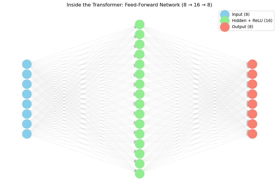
5.3. Visualising the Feed-Forward Network (FFN)
The Feed-Forward Network processes each token individually. It expands the 8 dimensions to 16 to find complex patterns, applies a ReLU activation, and shrinks it back to 8 dimensions. Since the network is small, we can plot every single node and connection using networkx and matplotlib.
plot_ffn_graph()
5.3.1. Position-wise Processing: Processing Token-by-Token (In Parallel)
The FFN does not look at the entire [4, 8] matrix at once. Instead, it treats the matrix as a list of four separate 8-dimensional vectors.
It applies the exact same \(8 \to 16 \to 8\) neural network to the 1st token, then to the 2nd token, then to the 3rd, and then to the 4th—completely independently.
In PyTorch, nn.Linear(8, 16) is smart enough to know that it should only operate on the very last dimension. It treats any dimensions before that (like our 4 tokens) as a batch.
5.3.2. The Matrix Multiplication Math
Because neural networks use matrix multiplication, this "token-by-token" processing happens all at once in a single, highly efficient calculation.
Here is how the shapes align perfectly during the first FFN step (Linear(8, 16)):
- Input Matrix (\(\mathbf{X}\)):
[4, 8](4 tokens, 8 features) - FFN Weight Matrix (\(\mathbf{W}_1\)):
[8, 16](8 inputs, 16 outputs)
When you multiply them (\(\mathbf{X} \times \mathbf{W}_1\)):
The output has shape [4, 16]. Each of the 4 tokens has been expanded from 8 dimensions to 16 dimensions using the same set of weights.
After the ReLU activation, the second linear layer (Linear(16, 8)) shrinks them back down: $\(\mathbf{O}_{\text{ffn}} = \text{ReLU}(\mathbf{X}_1 \mathbf{W}_1 + \mathbf{b}_1)\mathbf{W}_2 + \mathbf{b}_2 \in \mathbb{R}^{4 \times 8}\)$
print("Shape before FFN:", norm1_out.shape)
hidden_state = model.transformer.ffn[0](norm1_out)
print("Shape inside FFN (expanded):", hidden_state.shape)
ff_out = model.transformer.ffn(norm1_out)
print("Shape after FFN:", ff_out.shape)
Shape before FFN: torch.Size([1, 4, 8])
Shape inside FFN (expanded): torch.Size([1, 4, 16])
Shape after FFN: torch.Size([1, 4, 8])
5.3.3. Why do it this way?
You might wonder: If we are processing them separately, how do the words communicate?
They already did!
- Self-Attention is the only layer where tokens talk to each other and mix their data.
- The FFN is the layer where each token pauses to independently "digest" the new information it just received from the group.
By applying the exact same FFN weights to every position, the model learns universal rules for processing language, regardless of whether a word appears at the beginning or the end of a sentence.
5.3.4. The Feed-Forward Output
With the shape of the network clear, we can pass the normalised matrix through it and display the resulting 8-dimensional output.
# 1. Pass the normalised data through the FFN
ff_out = model.transformer.ffn(norm1_out)

visualise_ff_output(ff_out, sentence)
4. Feed-Forward Network Output:
| FFN_Out_1 | FFN_Out_2 | FFN_Out_3 | FFN_Out_4 | FFN_Out_5 | FFN_Out_6 | FFN_Out_7 | FFN_Out_8 | |
|---|---|---|---|---|---|---|---|---|
| < START > | 1.062 | -12.492 | 3.892 | -1.524 | 1.508 | 2.212 | -0.461 | 1.719 |
| i | 1.090 | -1.889 | 0.426 | -0.670 | 0.443 | -0.832 | 0.296 | -0.462 |
| am | 0.252 | -1.765 | 0.624 | -0.050 | 0.268 | -0.155 | 0.563 | 0.507 |
| groot | -0.261 | 1.693 | -1.950 | 0.668 | 2.212 | -1.157 | 3.153 | 1.382 |
Part 6: Logits, Probabilities, and Generation
We are at the final stretch. The Feed-Forward Network has processed our context, but it is still in an 8-dimensional internal format. We need to turn this back into human-readable words. 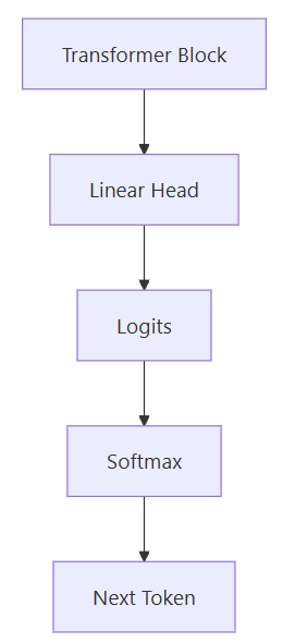
6.1. Second Residual & Final Normalisation
We add the FFN output back to its input (norm1_out) and normalise it one last time (norm2) to get the final hidden state for the block. $$ F = \text{FFN}(N_1), \quad R_2 = N_1 + F, \quad H_{\text{out}} = \text{LayerNorm}(R_2) $$
# 1. Second Residual Connection and Final Layer Normalisation
residual_2 = norm1_out + ff_out
final_block_out = model.transformer.norm2(residual_2)

display_final_block_out(final_block_out, residual_2, sentence)
1. Final Transformer Block Output (norm2):
| Final_Out_1 | Final_Out_2 | Final_Out_3 | Final_Out_4 | Final_Out_5 | Final_Out_6 | Final_Out_7 | Final_Out_8 | |
|---|---|---|---|---|---|---|---|---|
| < START > | 0.852 | -4.997 | 1.705 | -0.019 | 0.047 | 1.706 | -0.002 | 1.434 |
| i | 2.509 | -1.850 | -1.246 | -0.851 | -1.597 | -0.589 | 5.091 | -1.104 |
| am | -1.478 | -2.702 | 2.303 | 2.872 | -3.089 | 2.206 | -2.120 | 2.070 |
| groot | -1.536 | 1.758 | -4.087 | 1.506 | 3.010 | -3.065 | 1.347 | 0.836 |
6.2. The Linear Prediction Head (Logits)
A final linear layer (model.head) acts as a translator, projecting our 8-dimensional hidden state into 24 dimensions (one for every word in our vocabulary). These raw scores are called logits.
he final hidden representations are projected from the latent space \(\mathbb{R}^8\) into the full vocabulary space \(\mathbb{R}^{24}\):
We only care about the logits for the last token ("groot"), because we want to predict what comes next.
# 1. Project from 8 dimensions back to our 24-word vocabulary
logits = model.head(final_block_out)

# 2. Extract the prediction for the LAST token in our sequence (index 3 for "groot")
last_token_logits = logits[0, 3, :].detach().cpu().numpy()

# 3. Pair each logit with its corresponding vocabulary word
vocab_words = [id_to_token[i] for i in range(vocab_size)]
df_logits = pd.DataFrame({
    "Vocabulary Word": vocab_words,
    "Raw Logit Score": last_token_logits
})

show_top_five_highest_scores(df_logits)
2. Top 5 Raw Logit Scores for the next word:
| Vocabulary Word | Raw Logit Score | |
|---|---|---|
| 2 | < END > | 11.534508 |
| 10 | helps | 8.676242 |
| 15 | needs | 6.360995 |
| 19 | smiles | 3.422407 |
| 6 | cries | 3.418268 |
6.3. Softmax Probabilities
Finally, we apply the Softmax function to convert these raw logits into percentages, showing us exactly how confident the model is about its decision. $$ p(y_t = i \mid x_{\le t}) = \frac{e^{\text{logit}_i}}{\sum_j e^{\text{logit}_j}} $$
# 1. Convert raw logits to probabilities summing to 1.0
probabilities = torch.softmax(logits[0, 3, :], dim=-1)

show_final_probabilities(probabilities, df_logits)
3. Final Next-Word Probabilities:
| Vocabulary Word | Raw Logit Score | Probability | Probability (%) | |
|---|---|---|---|---|
| 2 | < END > | 11.534508 | 0.939936 | 93.99% |
| 10 | helps | 8.676242 | 0.053922 | 5.39% |
| 15 | needs | 6.360995 | 0.005324 | 0.53% |
| 19 | smiles | 3.422407 | 0.000282 | 0.03% |
| 6 | cries | 3.418268 | 0.000281 | 0.03% |
By looking at these tables, you can clearly trace how the abstract 8-dimensional array mathematically decodes into a 93.99% confidence that the sentence should end!
7. Final Output and summary
Language generation in GPT-style models is autoregressive and iterative. The model does not write an entire sentence in one shot. Instead, it generates one single token at a time in a loop:
- It reads whatever text you provide as a prompt.
- It predicts the most likely immediate next word.
- It appends that new word to the end of the prompt.
- It feeds this expanded sequence back into itself and repeats the process until it generates the
<END>token or hits a length limit.
In this step, we use Greedy Decoding (via argmax), which means the model always selects the token with the highest predicted score (logit). $\(\hat{y} = \operatorname{argmax}(\mathbf{z}_{\text{last}})\)$
def generate_argmax(prompt, max_new_tokens=5):
    model.eval()
    generated_ids = [token_to_id["<START>"]] + [token_to_id[token] for token in prompt.split()]

    for _ in range(max_new_tokens):
        active_ids = generated_ids[-max_len:]
        x = active_ids + [pad_id] * (max_len - len(active_ids))
        x_tensor = torch.tensor([x], device=device)

        with torch.no_grad():
            logits, _ = model(x_tensor)

        boundary_index = len(active_ids) - 1
        next_token_id = torch.argmax(logits[0, boundary_index]).item()
        generated_ids.append(next_token_id)

        if id_to_token[next_token_id] == "<END>":
            break

    return " ".join(id_to_token[token_id] for token_id in generated_ids)
7.1 I am Groot
Now trace what happens when we prompt the model with "i am".
- Prompt:
"i am" - This gets converted to Initial Token IDs:
['<START>', 'i', 'am'] - Target Maximum Length (\(T_{\max}\)): \(4\)
7.1.1 Iteration 1: Predicting Token 1
- Input Vector is Padded to 4): "
", "i", "am", " "} - Extracted Logits Matrix (\(\mathbf{z}_{\text{next}}\) at Index 2): The model computes scores for all 24 vocabulary words at position 2 (following
"am"). The highest score is at index 8, which corresponds to"groot") - Updated Sequence:
['<START>', 'i', 'am', 'groot']
7.1.2 Iteration 2: Predicting Token 2
- Input Vector: "
", "i", "am", "groot" - Extracted Logits Matrix (\(\mathbf{z}_{\text{next}}\) at Index 3): The model computes scores at position 3. The highest score is at index 2, which corresponds to
"<END>" - Stop Condition Triggered: Token
2is"<END>". The generation loop halts.
Final Generated Output:
"<START> i am groot <END>"
print(generate_argmax("i am"))
<START> i am groot <END>
7.2 Other Generation Examples from the Model:
print(generate_argmax("groot likes"))
print(generate_argmax("tree needs"))
print(generate_argmax("rocket helps"))
<START> groot likes leaf <END>
<START> tree needs water <END>
<START> rocket helps rocket <END>
7.3 Summary
The following short notes add context for related concepts:
Single-Head vs Multi-Head Attention For simplicity, BabyGrootGPT uses a single attention head. In production models like GPT-2, the embedding dimension is split across multiple heads that run in parallel. This Multi-Head Attention allows the model to capture different linguistic relationships simultaneously—for example, one head might focus on grammatical structure while another tracks contextual meaning—before concatenating the results back together.
Pre-Layer vs Post-Layer Normalisation You might notice that our Transformer block applies Layer Normalisation after the residual addition (x = self.norm1(x + attn_out)), matching the architecture from the original "Attention is All You Need" paper. However, modern architectures like GPT-2 typically use Pre-LN, applying normalisation before the attention and feed-forward blocks to improve training stability at massive scales.
Positional Embedding Strategy We use a simple learned lookup table (nn.Embedding) to give our model a sense of position. While the original Transformer paper used fixed, mathematical sinusoidal waves to encode token positions, modern decoder-only models like GPT often opt for learned positional embeddings exactly like ours, letting the model figure out spatial relationships directly from the training data.
Decoding Strategies: Argmax vs Sampling Our text generation loop uses greedy decoding via argmax, meaning it always picks the single most likely next token. While straightforward, greedy decoding often causes models to get stuck in repetitive, infinite loops. Real-world language models solve this by using Temperature and Top-K/Top-P sampling, which introduce controlled randomness into the token selection to produce more creative and natural-sounding text.
The Batch Dimension in Matrix Operations Throughout our matrix walkthrough, we traced a single sequence resulting in a shape of [1, 4, 8]. During actual training, however, models process many sequences at once by utilizing a batch dimension. This makes the true tensor shape \(B \times T \times C\) (Batch \(\times\) Time \(\times\) Channel), allowing neural networks to leverage highly optimized parallel matrix multiplications across thousands of examples simultaneously.
Overall flow diagram 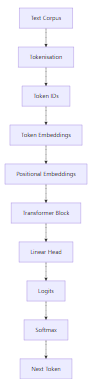
Deep dive flow diagram 
Deep dive flow diagram