Backpropagation
Introduction
This is the second in a series of blogs about neural networks. In this blog, we will discuss and implement the backpropagation algorithm from scratch. In the previous blog, we have seen how a single perceptron works when the data is linearly separable. In this blog, we will look at the workings of a multi-layered perceptron (with theory) and understand the maths behind backpropagation.
Multi-layer perceptron
An MLP is composed of one input layer, one or more layers of perceptrons called hidden layers, and one final perceptron layer called the output layer. Every layer except the input layer is connected with a bias neuron and is fully connected to the next layer.
Perceptron
In the previous blog, we saw a perceptron with a single TLU. A Perceptron with two inputs and three outputs is shown below. Generally, an extra bias feature is added as input. It represents a particular type of neuron called a bias neuron. A bias neuron outputs one all the time. This layer of TLUs is called a perceptron.
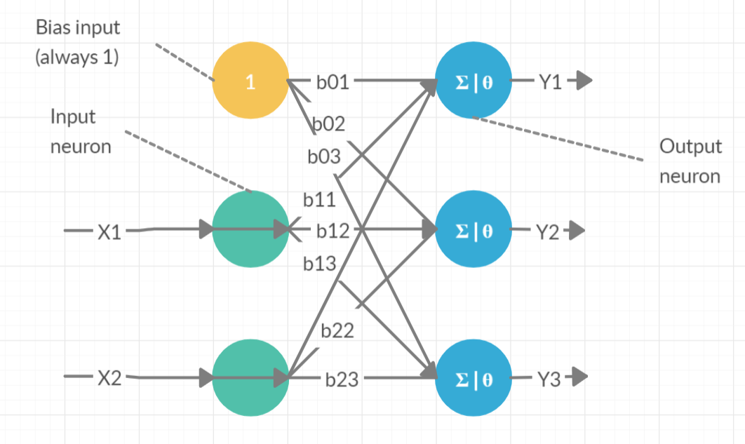
In the above perceptron, the inputs are x1 and x2. The outputs are y1, y2 and y3. Θ (or f) is the activation function. In the last blog, the step function is taken as the activation function. There are other activation functions such as:
Sigmoid function: It is S-shaped, continuous and differentiable where the output ranges from 0 to 1.
$$ f(z)=\frac{1}{1+e^{-z}} $$
Hyperbolic Tangent function: It is S-shaped, continuous and differentiable where the output ranges from -1 to 1. $$ f\left(z\right)=Tanh\left(z\right) $$
ReLU: Rectified Linear Unit function or ReLU is continuous but not differentiable at z=0. It can be defined as max(z,0), so it is zero for all negative values of z, and linear for all positive values. $$ f(z) = max(z,0) $$
Training
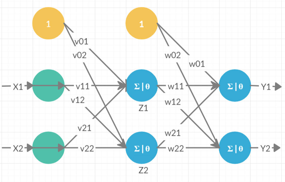
Training a network in ANN has three stages, feedforward of input training pattern, backpropagation of the error and adjustment of weights. Let us understand it using a simple example. Consider a simple two-layered perceptron as shown:
Nomenclature
| Symbol | Meaning | Symbol | Meaning |
|---|---|---|---|
| \(X_i\) | Input neuron | \(Y_k\) | Output neuron |
| \(x_i\) | Input value | \(y_k\) or \(y_{actual}\) | Output value |
| \(Z_j\) | Hidden neuron | \(z_j\) | The output of a hidden neuron |
| \(w_{jk}\) | Weight of j to k | \(v_{ij}\) | weight of i to j |
| \(\theta_k\) | Error propagating from \(Y_k\) to \(Z_k\) | \(\theta_j\) | Error propagating from \(Z_k\) to \(X_k\) |
| \(\delta_k\) | The portion of error correction for weight \(w_{jk}\) | \(\delta_j\) | The portion of error correction for weight \(v_{ij}\) |
| \(\alpha\) | Learning rate | \(t_j\) or \(y_{pred}\) | Predicted output |
| f | Activation function | -- | -- |
Initialising
import numpy as np
import matplotlib.pyplot as plt
import random
np.random.seed(42)
num_inputs = 50
input_dimension = 2
hidden_layer_dimension = 2
output_dimension = 2
alpha=0.1
Let us consider the sigmoid function as an activation function and create input and output values.
# Sigmoid function
def sigmoid(model_output):
    return 1/(1 + np.exp(-model_output))

# Creating random input values
x = np.array([[random.random(), random.random()] for x in range(num_inputs)])

# Creating output values
y_actual = sigmoid(sigmoid(x)+random.random()*0.1)+random.random()*0.1

# The first input to the model is
x[0]
array([0.17988842, 0.42611707])
Adding a bias neuron
bias = np.ones((num_inputs, 1))
x_bias = np.hstack((bias, x))

# Adding the bias, the input becomes
x_bias[0]
array([1. , 0.17988842, 0.42611707])
Creating the hidden layer and initialising weights with random numbers
v = np.random.randn(input_dimension+1,hidden_layer_dimension)

# Inital weights are
v
array([[ 0.49671415, -0.1382643 ],
       [ 0.64768854,  1.52302986],
       [-0.23415337, -0.23413696]])
Creating the output layer and initialising weights with random numbers
w = np.random.randn(hidden_layer_dimension+1,output_dimension)

# Hidden layer weights are
w
array([[ 1.57921282,  0.76743473],
       [-0.46947439,  0.54256004],
       [-0.46341769, -0.46572975]])
Feedforward loop
During feedforward, each input unit \(X_i\) receives input and broadcasts the signal to each of the hidden units \(Z_1\ldots Z_j\). Each hidden unit then computes its activation and sends its signal (\(z_j\)) to each output unit. Each output unit \(Y_k\) computes its activation (\(y_k\)) to form the response to the input pattern.
Input layer
Step 1. Each input unit (\(X_i\)) receives the input \(x_i\) and broadcasts this signal to all units to the hidden layers \(Z_j\).
Hidden layer
Step 2. Each hidden unit (\(Z_j\)) sums its weighted input signals \(z\_in_j=v_{0j}+\sum_{i} x_i\times v_{ij}\)
Z_input = x_bias.dot(v)

# Input to the hidden layer
Z_input[0]
array([0.51344907, 0.03594138])
Step 3. The activation function is applied to this weighted sum to get the output. \(z_j=f\left(z\_in_j\right)\) (where f is the activation function).
z = sigmoid(Z_input)
z_bias = np.hstack((bias, z))

# Output in the hidden layer
z_bias[0]
array([1. , 0.62561467, 0.50898438])
Step 4. Each hidden layer sends this signal (\(z_j\)) to the output layers.
Output layer
step 5. Each output unit (\(Y_k\)) sums its weighted input signals \(y\_in_k=w_{0k}+\sum_{j}z_j\times w_{jk}\)
Y_input = z_bias.dot(w)

# Input to output layer
Y_input[0]
array([1.04963039, 0.86981908])
Step 6. The activation function is applied to this weighted sum to get the output. \(y_k=f\left(y\_in_k\right)\) (where f is the activation function).
y_pred = sigmoid(Y_input)

# Predicted output
y_pred[0]
array([0.74070392, 0.70470805])
Backpropagation of error
During training, each output unit \(Y_k\) compares its predicted output \(y_k\) with its actual output \(t_k\) to determine the error associated with that unit. Based on this error, \(\delta_k\) is computed. This \(\delta_k\) is used to distribute the error at the output unit back to all input units in the previous layers. Similarly, \(\delta_j\) is computed for all hidden layers \(Z_j\) which is propagated to the input layer.
Output layer
Step 7. The error information term (\(\theta_k\)) is computed at every output unit (\(Y_k\)). $$ \theta_k=\left(t_k-y_k\right)f’ $$ $$ \delta_k=\left(t_k-y_k\right)f’ y_in_k $$
Note: \(f’(z) = \frac{d}{dz}(\frac{1}{1+e^{-z}}) = f(z)\times(1-f(z))\)
theta_k = (y_pred - y_actual)*(y_pred*(1-y_pred))
delta_k = z_bias.T.dot(theta_k)

# Error that has to backpropogated in output layer
delta_k[0]
array([0.54340751, 0.28015272])
Step 8. This error is propagated back to the hidden layer. (later weights will be updated using this \(\delta\))
Hidden layer
Step 9. Each hidden unit (\(Z_j\)) sums its weighted error from the output layer $$ \theta_in_j=\sum_{k}\theta_k\times w_{jk} $$
theta_in_j = theta_k.dot(w[1:])

# Error split across weights
theta_in_j[0]
array([-0.01210996, 0.00547047])
Step 10. The derivative of the activation function is multiplied by this weighted sum to get the weighted error information term at the hidden layer. $$ \theta_j=\theta_in_j \times f^\prime $$ $$ \delta_j=\delta_in_j \times f^\prime\left(z_in_j\right) $$
theta_j = theta_in_j*(z*(1-z))
delta_j = x_bias.T.dot(theta_j)


# Error that has to be backpropogated in hidden layer
delta_j[0]
array([-0.08582196, 0.03962274])
Step 11. This error is propagated back to the initial layer.
Update weights and biases
The \(\delta_k\) and \(\delta_j\) are used to update the weights \(w_{jk}\) and \(v_{ij}\) respectively. The weight adjustment is based on gradient descent and is dependent on error gradient (\(\delta\)), learning rate (\(\alpha\)) and input to the neuron.
Step 12. The weights are updated based on the error information terms $$ w_{jk}\left(new\right)=w_{jk}\left(old\right)+\Delta w_{jk} $$ where $ \Delta w_{jk}=\alpha\times\delta_k\times z_j $
$$ v_{ij}\left(new\right)=v_{ij}\left(old\right)+\Delta v_{ij} $$ where $ \Delta v_{ij}=\alpha\times\delta_j\times x_i $
# Updating weights
w = w - alpha*delta_k
v = v - alpha*delta_j
Gradient descent and training
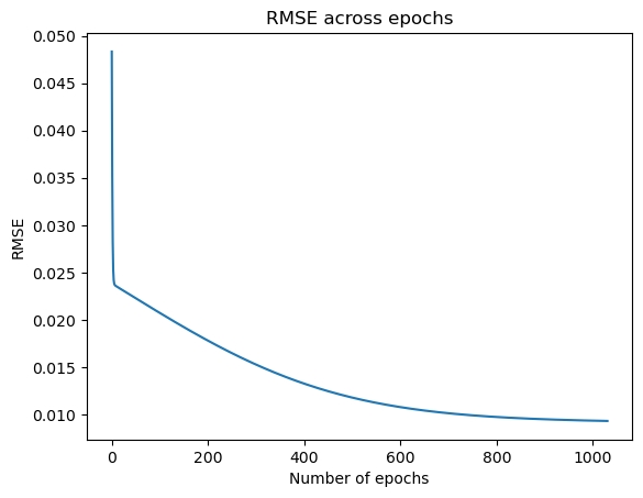
Gradient descent is an iterative optimization algorithm for finding the minimum of a function; in our case, we want to minimize the error function. To find a local minimum of a function using gradient descent, one takes steps proportional to the negative of the gradient of the function at the current point. This means training steps 1-12 are done for each training epoch until a stopping criterion is met.
Stopping criterion: Difference in error between the previous epoch and current epoch is at least greater than 0.00001
# Repeat for 10000 iterations or stop at stopping criterion
error = y_actual - y_pred
rmse = np.sqrt((error** 2).mean())
error_array = [rmse]
for i in range(10000):
    # Feedforward loop
    Z_input = x_bias.dot(v)
    z = sigmoid(Z_input)
    z_bias = np.hstack((bias, z))
    Y_input = z_bias.dot(w)
    y_pred = sigmoid(Y_input)

    # Backpropogation
    theta_k = (y_pred - y_actual)*(y_pred*(1-y_pred))
    delta_k = z_bias.T.dot(theta_k)
    theta_in_j = theta_k.dot(w[1:])
    theta_j = theta_in_j*(z*(1-z))
    delta_j = x_bias.T.dot(theta_j)
    w = w - alpha*delta_k
    v = v - alpha*delta_j

    # Calculating error
    error = y_actual - y_pred
    rmse = np.sqrt((error** 2).mean())
#     print(i, rmse)

    error_array.append(rmse)
    if((i>1) & (abs(rmse-error_array[-2])<0.000001)):
        plt.plot(list(range(len(error_array))), error_array)
        plt.title('RMSE across epochs')
        plt.xlabel('Number of epochs')
        plt.ylabel('RMSE')
        plt.show();
        break
Prediction and accuracy
Using the updated weights, we can predict the values for any new data point.
def prediction(x_pred):
    bias_ = np.ones((len(x_pred), 1))
    return sigmoid(np.hstack((bias_, sigmoid(np.hstack((bias_, x_pred)).dot(v)))).dot(w))
prediction(x[0:1])
array([[0.65845299, 0.67733945]])
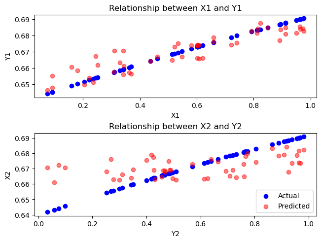
Actual vs predicted variables are also plotted below
fs, axs = plt.subplots(2, gridspec_kw={'height_ratios': [1,1]}, constrained_layout=True)
axs[0].scatter(x.T[0], y_actual.T[0], color='blue')
axs[0].scatter(x.T[0], y_pred.T[0], color='red', alpha=0.5)

axs[1].scatter(x.T[1], y_actual.T[1], color='blue', label='Actual')
axs[1].scatter(x.T[1], y_pred.T[1], color='red', alpha=0.5, label='Predicted')

# plt.title('Actual vs prediction')

axs[0].set_ylabel('Y1')
axs[0].set_xlabel('X1')
axs[0].set_title('Relationship between X1 and Y1')
axs[1].set_ylabel('X2')
axs[1].set_xlabel('Y2')
axs[1].set_title('Relationship between X2 and Y2')
plt.legend(loc='lower right')
plt.show();
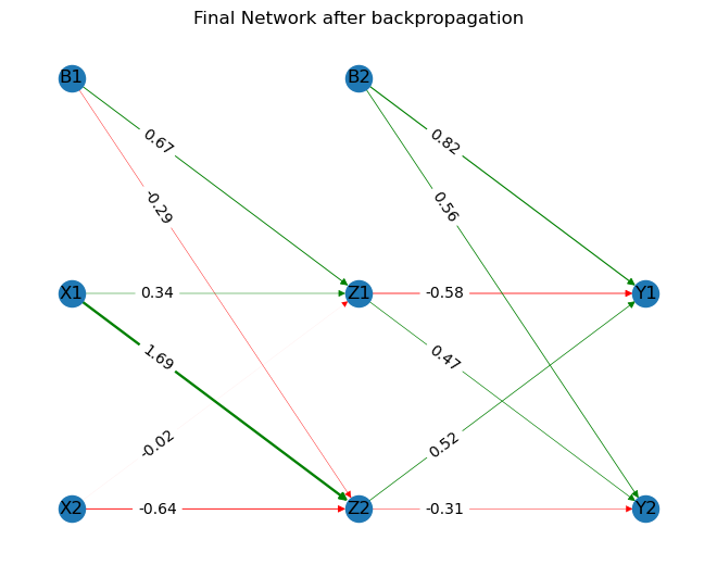
The final network along with its weights can be plotted using networkx.
import networkx as nx
import pandas as pd
g = nx.DiGraph()
edgelist_df = pd.DataFrame({
    'node1':['B1', 'B1', 'X1', 'X1', 'X2', 'X2', 'B2', 'B2', 'Z1', 'Z1', 'Z2', 'Z2'],
    'node2':['Z1', 'Z2', 'Z1', 'Z2', 'Z1', 'Z2', 'Y1', 'Y2', 'Y1', 'Y2', 'Y1', 'Y2'],
    'weights':[ '%.2f' % elem for elem in np.hstack((v.flatten() ,w.flatten()))],
    'width':np.hstack((v.flatten() ,w.flatten())),
    'color': ['green' if val>0 else 'red' for val in np.hstack((v.flatten() ,w.flatten()))]
                           })
g = nx.DiGraph()
for i, elrow in edgelist_df.iterrows():
    g.add_edge(elrow[0], elrow[1], weight=elrow[2], width=elrow[3], color=elrow[4])
g.add_node('X1',pos=(0,2))
g.add_node('X2',pos=(0,1))
g.add_node('B1',pos=(0,3))
g.add_node('Z1',pos=(1,2))
g.add_node('Z2',pos=(1,1))
g.add_node('B2',pos=(1,3))
g.add_node('Y1',pos=(2,2))
g.add_node('Y2',pos=(2,1))
g.nodes(data=True)

# This function gets the weights for the edges
weight = nx.get_edge_attributes(g,'weight')
pos = nx.get_node_attributes(g,'pos')
width = nx.get_edge_attributes(g,'width')
color = nx.get_edge_attributes(g,'color')
color = [color[val] for val in color]
width = [abs(width[val]) for val in width]

# nx.draw(g,pos, with_labels=True, edge_color= color, width=abs(np.hstack((v.flatten() ,w.flatten()))))
nx.draw(g,pos, with_labels=True, edge_color = color, width=width)
nx.draw_networkx_edge_labels(g,pos,edge_labels = weight, label_pos=0.7)
plt.title('Final Network after backpropagation')
plt.show()
Derivation of learning rules
In every loop while training, we change the weights (\(v_{ij}\) and \(w_{jk}\)) to find the optimal solution. What we want to do is to find the effect of changing the weights on the error, and minimise the error using gradient descent.
The error gradient that has to be minimised is given by: $$ E=\frac{1}{2}\sum_{k}\left(t_k-y_k\right)^2 $$ The effect of changing an outer layer weight (\(w_{jk}\)) on the error is given by: $$ \frac{\partial E}{\partial w_{jk}}=\frac{\partial}{\partial w_{jk}}\frac{1}{2}\sum_{k}\left(t_k-y_k\right)^2 $$ $$ =\left(y_k-t_k\right)\frac{\partial}{\partial w_{jk}}f\left(y_in_k\right) $$ $$ =\left(y_k-t_k\right)\times z_j\times f'\left(y_in_k\right) $$ Therefore $$ \Delta w_{jk}=\alpha\frac{\partial E}{\partial w_{jk}}=\alpha\times\left(y_k-t_k\right)\times z_j\times f^\prime\left(y_in_k\right)={\alpha\times\delta}_k\times z_j $$
The effect of changing the weight of a hidden layer weight (\(v_{ij}\)) on the error is given by:
$$ \frac{\partial E}{\partial v_{ij}}=\sum_{k}{\left(y_k-t_k\right)\frac{\partial}{\partial v_{ij}}f\left(y_k\right)} $$ $$ =\sum_{k}\left(y_k-t_k\right)f^\prime\left(y_in_k\right)\frac{\partial}{\partial v_{ij}}f\left(y_k\right) $$ $$ =\sum_{k}\delta_kf^\prime\left(z_in_j\right)\left[x_i\right] =\delta_j\times x_i $$ Therefore $$ \Delta v_{ij}=\alpha\frac{\partial E}{\partial v_{ij}}={\alpha\times\delta}_j\times x_i $$ This way, for any number of layers, we can find the error information terms. Using gradient descent, we can minimise the error and find optimal weights for the ANN. In the next blog, we will discuss tensorflow and keras.
References
- Fausett, L., 1994. Fundamentals of neural networks: architectures, algorithms, and applications. Prentice-Hall, Inc.
- https://mattmazur.com/2015/03/17/a-step-by-step-backpropagation-example/
- GeÌron, A. (2019). Hands-on machine learning with Scikit-Learn, Keras and TensorFlow: concepts, tools, and techniques to build intelligent systems (2nd ed.). O’Reilly.
- Class notes: Business Analytics & Intelligence (BAI –10): Prof Naveen Kumar Bhansali