Perceptron

Introduction¶

In this series of posts, I would like to create an artificial neural network from scratch. In this post, I would like to give an introduction to human neurons and a comparison to ANN. Using a single-layered perceptron model, I will try to solve a linearly separable problem.

Artificial neural networks are the backbone of artificial intelligence and deep learning. They are versatile and scalable, making them ideal for tackling complex tasks like image classification, speech recognition, recommendation systems and natural language processing.

Biological vs Artificial Neurons¶

We are trying to imitate the functioning of the brain. Although we don't exactly know what exactly happens in the brain, we have a basic understanding. We are trying to approximate it using mathematical functions.
The human brain has billions of neurons. In humans, neurons are a network of 100 million neurons and 60 trillion connections. If each neuron is approximated to a computing unit, this cannot be replicated currently by computers.

In the human brain, a neuron consists of different parts:
Soma: The cell body (Approximated to the neuron in ANN)
Dendrites: Input to the cell (Approximated to the input)
Synopses: It is the weight assigned to the input (Approximated to the weight or slope)
Axon: Output to a neuron (Approximated to the final output)

What happens in a neuron?¶

When a neuron receives signals from different dendrites, the signals are cumulated. In a simplified understanding, if this cumulated signal is greater than a certain value, it passes these signals to the next neuron. Neuron, when it communicates with neighbouring neurons, it uses electrochemical reactions which are approximated to a mathematical function called the activation function.

In humans, neurons have computing powers as well as cognition powers. Also, the human brain neural network is plastic, which means, some neurons die, new neurons are created, the synapses change, etc.
[1]

How do we approximate it to an ANN¶

In an Artificial neuron, the soma is approximated to the neuron. The dendrites are the input function, the synapses are the weights and the Axon is approximated to an output. A representation of a neuron (also called TLU) is below:
TLU sample

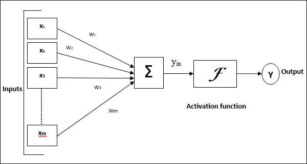
Activation function: In biological systems, the neurons transmit signals after they reach some threshold potential. The below figure shows how the neuron transmits the signal only after the signal is greater than the threshold potential. In ANN, this is mathematically represented using an activation function. Please see this link for understanding: Action potential propagation

Perceptron¶

The perceptron is the simplest ANN architecture. A perceptron contains a single layer of TLU(Threshold Logical Units). The input and outputs are numbers, and each of the inputs has a weight. A weighted sum of the inputs is computed (z), and then an activation function is applied to get the result (y).
$$ z = w_1 \times x_1 + w_2 \times x_2 ... w_n \times x_n $$ In the current example, the step function is the activation function. If the data is mutually separable, a step function is sufficient for classification problems.

\[ step(z) =\begin{cases} -1 & z < \theta \\ 0 & z = \theta \\ 1 & z > \theta \end{cases} \]

Also, ANNs are models from where simple business understandable rules cannot be generated, which creates a reluctance for its widespread use when other explainable models can be used.

A perceptron model has four steps:

Step 1: Set initial weights $w_1, w_2 ... w_n$ and threshold $\theta$ (bias). We generally take small values between [-0.5, 0.5]
Step 2: Identify the activation function
Step 3: Weight training: Weight is updated based on error: The weight correction is done based on the error. The weight in node i is the previous weight plus an additional correction. This correction is a product of learning rate, input value and error. $$ w_i(p+1) = w_i(p) + \delta w_i(p) $$ $$ \delta w_i(p) = \alpha \times x_i(p) \times e(p) $$

Where $w_i(p)$ is the weight at step p correction and $\alpha$ is the learning rate.

Step 4: Repeat till stopping criterion

Even with such a simple model, we can train the model to perform logical computations like or-gate. The input and output for an and-gate are as follows:

# Loading packages and initialising
import numpy as np
import matplotlib.pyplot as plt
np.random.seed(42)
num_inputs = 4
dimension = 2
alpha=0.1

input 1	input 2	output
0	0	0
0	1	1
1	0	1
1	1	1

input_array = np.array([
    [0, 0],
    [0, 1],
    [1, 0],
    [1, 1],
])
output_array = np.array([0, 1, 1, 1])

A single-layer simple TLU is taken to solve this problem. 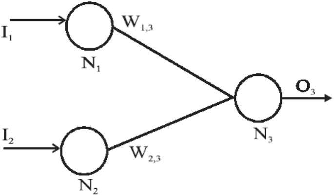single layer perceptron

Step 1:¶

Randomly choosing weights of $w_{1,3} = 0.49$, $w_{2,3} = -0.13$,

# randomly initialize the weights
weight = np.random.randn(dimension)
weight

array([ 0.49671415, -0.1382643 ])

Step 2:¶

The activation function is the step function which is described above.
$$ step(z) =\begin{cases} 0 & z \leq 0 \ 1 & z > 0 \end{cases} $$

For the above weights, The output for the four scenarios is:

Output for epoch 1
input 1 ($I_1$)	input 2 ($I_2$)	$w_{1,3}$	$w_{2,3}$	input to N3	output ($O_3$)
0	0	0.49	-0.13	0	0
0	1	0.49	-0.13	00.49+1(-0.13) = -0.13	step(-0.13)=0
1	0	0.49	-0.13	10.49+0(-0.13) = 0.49	step(0.49) = 1
1	1	0.49	-0.13	10.49+1(-0.13) = 0.36	step(0.36) = 1

model_output = input_array.dot(weight)
y_pred = np.heaviside(model_output, 0)
y_pred

array([0., 0., 1., 1.])

Step 3:¶

Weight training: Weight is updated based on error: The weight correction is done based on the error. The weight in node i is the previous weight plus an additional correction. This correction is a product of learning rate, input value and error. $$ w_i(p+1) = w_i(p) + \delta w_i(p) $$ $$ \delta w_i(p) = \alpha \times x_i(p) \times e(p) $$

Where $w_i(p)$ is the weight at step p correction and $\alpha$ is the learning rate.
assuming a $\alpha=0.1$, we have the following values

Error for epoch 1
input 1 ($I_1$)	input 2 ($I_2$)	Pred ($O_3$)	Actual output	Error ($\epsilon$)	$\delta w_{1,3}$	$\delta w_{2,3}$
0	0	0	0	0	0	0
0	1	0	1	1	$\delta w_{1,3}(2) = \alpha \times I_1(2) \times e(2) = 0.1\times 0\times 1 = 0$	$\delta w_{2,3}(2) = \alpha \times I_2(2) \times e(2) = 0.1\times 1\times 1 = 0.1$
0	1	1	1	0	0	0
1	1	1	1	0	0	0

Therefore the updated weights are $w_{1,3} = 0.49, w_{2,3} = -0.03$

weight + alpha*input_array.T.dot(output_array - y_pred)

array([ 0.49671415, -0.0382643 ])

Step 4¶

One such iteration is called an epoch. For the optimal neural network, we should run different epochs until the errors (also called cost function) are zero (near zero). As this is a linearly separable case, the stopping criterion is that the error is zero.

error = output_array - y_pred
error_array = []
while ~(error == np.zeros(4)).all(): # stopping criterion is zero
    # Step 2
    error = output_array - y_pred
    # Step 3
    weight += alpha*input_array.T.dot(error)

    # Step 1
    model_output = input_array.dot(weight)
    y_pred = np.heaviside(model_output,0)

    rmse = np.sqrt((error** 2).mean())
    print('weights:', weight, ' rmse:', rmse)
    error_array.append(rmse)

weights: [ 0.49671415 -0.0382643 ]  rmse: 0.5
weights: [0.49671415 0.0617357 ]  rmse: 0.5
weights: [0.49671415 0.0617357 ]  rmse: 0.0

The decision boundary for the same is given as

fs, axs = plt.subplots(1)
plt.plot([weight[0], 0], [0, weight[1]])
for i in range(len(input_array)):
    axs.annotate(
        input_array[i], 
        xy=input_array[i], 
        xytext=input_array[i]
    )
plt.xlim([0,1.1])
plt.ylim([0,1.1])
plt.xlabel('X1')
plt.ylabel('X2')
plt.title('OR gate and decision boundary using a Perceptron')
plt.show();

png

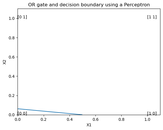
After 4^th epoch, the error is zero. The final weights are $w_{1,3} = 0.49$ and $w_{2,3} = 0.06$

The second blog is on backpropagation.